


1. Introduction
Subaerial and submarine landslides, mainly caused by heavy rain or earthquake, play a crucial role in numerous disasters. Subaerial landslide or debris flow on the earth surface caused extremely hazard events in the landslide histories (Jakob et al., 2000; McDougall et al., 2006; Van Tien et al., 2018). Also submarine landslide was mentioned to be one of significant contributions to the generation of enormous tsunamis in coastal zones (Horrillo et al., 2013; Sassa et al., 2016; Tappin et al., 2014). In recent decades, lots of efforts have been made to investigate the behavior of landslides using laboratory experiments (Iverson, 2003, 2015; Iverson et al., 2010; Major, 1997) or numerical simulations (Denlinger and Iverson, 2001; Imran et al., 2001; McDougall et al., 2006; Naef et al., 2006) due to difficulties in measuring the field data. Numerical model results were compared with the real-time field events for verification of the model. The model with the shallow water equations was often used for landslide or debris flow simulation. Paik (2015) used a high-resolution finite volume scheme in the shallow water equations for modeling debris flow. The model results were in good agreement with both the analytical solution and the experimental data even near the wet and dry front. Yavari-Ramshe et al. (2015) introduced a robust finite volume model based on the shallow water equations to simulate granular flows. The numerical solutions were compared to experimental data with a relative error less than 5%. The finite volume method (FVM) is known to be suitable for discretizing the shallow water equations. Using a conservative form of the governing equations, the finite volume method can deal with numerical discontinuities like shock or dry/wet front in hydraulic engineering problems (Erduran et al., 2002).
In this study, we develop a subaerial and submarine landslide model using the shallow water equations with the coordinate of (b, s). Here b and s are vertical locations from a reference line. In river flow or debris flow, people often use the Saint-Venant equations with the variable of depth of water or debris instead of b and s. When using the shallow water equations with the coordinate of (b, s), it is possible to simulate flow in river and coastal zones simultaneously. We use the finite volume method to discretize the governing equations to deal with numerical discontinuities. In section 2, we develop a model of subaerial and submarine landslides based on the shallow water equations with the coordinate of (b, s) and the finite volume method is used to discretize the governing equations. In section 3, we validate the developed model by comparing numerical results with analytical solutions and experimental data for dambreak water flow and debris flow. In section 4, we apply the developed model to subaerial and submarine landslides and find reasonable results. In section 5, we summarize the present investigation and suggest future study.
2. Development of Landslide Model
In this section, a model of subaerial and submarine landslides is developed based on the shallow water equations with the coordinate of (b, s) and the finite volume method is used to discretize the governing equations.
2.1 Derivation of governing equations
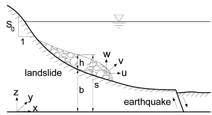
Fig. 1 shows the computational domain for simulating submarine landslide and defined variables. In the figure, s and b are the elevations of the surface and bottom of the debris from a reference line, h (= s − b) is the debris depth, and (u, v, w) are the velocities in the (x, y, z) directions. The continuity equation for the incompressible fluid flow is given by
Boundary conditions at the surface and bottom of the debris are as follows:
We integrate Eq. (1) from the bottom to the surface and use the Leibnitz’s rule with the boundary conditions given by Eqs. (2) and (3). Finally, we get the continuity equation in two-dimensional (x, y) domain as
and the continuity equation in one-dimensional (x) domain as
The x-directional momentum equation is defined as follows:
where τxx, τyx, τzx are the shear stresses. We only consider the x − z plain, so τxx, τyx are equal zero. In Eq. (6), the pressure p is assumed to be hydrostatic and thus p= ρg(s − z). We add u(∂u/∂x + ∂v/∂y + ∂w/∂z) to Eq. (6) in order to get the following equation
where − ∂b/∂x(= S0) is the bottom slope. We integrate Eq. (7) from the bottom to the surface, use the Leibnitz’s rule and the boundary conditions given by Eqs. (2) and (3). After neglecting the shear stress at the free surface, the resulting momentum equation is given as
In one-dimensional (x) domain, Eq. (8) is reduced to
which can also be expressed as
using the following relation as τ z x z = b = ρ g ( s - b ) S f
where n and μ are the Manning’s roughness and the effective friction coefficients, respectively. Manning’s n values range from 0.032 to 0.2 s/m1/3 while the μ values for debris flows range from 0.06 to 0.175 (Paik, 2015).
Eqs. (5) and (10) are the one-dimensional shallow water equations in a conservative form to deal with numerical discontinuities in landslides. Using chain rule and the continuity Eq. (5), the momentum Eq. (10) becomes
and, further dividing by (s − b), the resulting momentum equation is given by
(Eqs. (5) and (13) are the one-dimensional shallow water equations in an alternative conservation form (Toro, 2001).
2.2 Numerical scheme
In the present model, a finite volume scheme with an approximate Riemann solver is used to discretize the governing equations in time. The governing equations of the one-dimensional shallow water equations can be written in a conservative form as
where
and U is the vector of conserved variables. (Eq. (14) is solved using the splitting method. At the first step, the homogenous pure advection problems are solved as
where the superscript “n” implies the present time step and the subscript “i” implies the cell center of the computational domain. At the second step, the final solutions of U are obtained by adding the source terms as
where U i ( s )
The WAF (weighted average flux) method is known as the second-order extension of the Godunov method. A TVD (total variation diminishing) version of the WAF method which results in a high-resolution method is employed in this study. Thus, the numerical flux at the cell interface can be expressed as
where ck(= SkΔt/Δx) is the Courant number related to the wave speed Sk. The flux jump across wave k at the cell interface is given by
and the WAF limiter function is given by
where
and r(k) is the ratio of the upwind change to the local change. B(r(k)) is the limiter function (Toro, 2001). In this study, we use the van Leer limiter function for B(r) as
The HLL approximate Riemann solver is used to determine the HLL numerical flux as
The wave speed estimates are given as
In Eq. (28), a K = g ( s K - b K )
where
For wet/dry bed conditions, the wave speeds are determined as
2.3 CFL criterion
The numerical scheme used in this study is explicit and the CFL (Courant-Friedrichs-Lewy) number is investigated for numerical stability. The speed of landslides, especially for the wet/dry front speed, can be affected by the friction slope terms. In this study, we use a new CFL criterion (Paik, 2015) to determine the time step given by
where c is the celerity, uf is the total friction velocity. In the Voellmy resistance relation, the total friction velocity can be expressed as
The value of 0.9 of the CFL number is used for all the simulations in this study.
3. Model Validation for Water Flow and Debris Flow
3.1 Validation for water flow after dam break
In the first part, we validate conservative forms of the equations for a dam-break problem. We compare solutions of conservative forms of the governing Eqs. (5) and (10) and alternative conservative forms of the governing Eqs. (5) and (13) using homogeneous parts of these equations. The computational domain is 2 m long, a dam is located in the middle of the domain and water of 0.1 m depth is located behind the dam. Figs. 2(a) and 2(b) show numerical solutions of water surface elevations at t = 0.2 s using the conservative forms and alternative conservative forms, respectively. In the figures, analytical solutions (Mangeney et al., 2000) as well as initial conditions are shown for comparison. The conservative forms of the equations yield the same solutions as the analytical solutions. However, the alternative conservative forms of the equations yield different solutions. At a point of dry bed, (s − b) is equal to zero. In deriving alternative conservative forms of the momentum Eq. (13), we divide some terms by zero-valued (s − b) which is mathematically meaningless. That is why numerical solutions of alternative form of the equations are different from the analytical solution in the dry/wet discontinuity points. In further investigation, we use the conservative forms of the equations only.
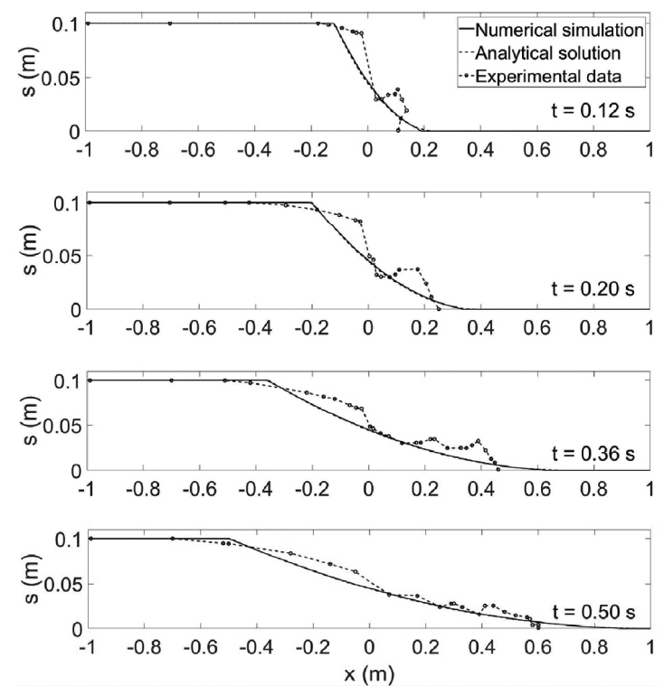
In the second part, we compare our model results with two cases with physical experimental data for water flow after dam break. The first case was done by Stansby et al. (1998). The test conditions are the same as in the first part. That is, the domain is 2 m long, a dam is located in the middle, and water with 0.1 m depth is located behind the dam. Fig. 3 compares numerical solutions, analytical solutions, and the measured data at t = 0.12 s, 0.20 s, 0.36 s, 0.50 s. On the whole, the numerical results show good agreements with the analytical solutions and the experimental data even though wave breaking occurred in reality. Especially, the numerical solutions are closer to the measured data at t = 0.36 s and t = 0.50 s when the water surface elevations are milder than at previous times.
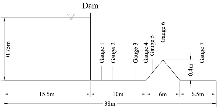
The second case was done by Liang and Marche (2009) who tested a large-scale dam-break flow over a symmetric triangular hump as shown in Fig. 4. The domain is 38m long and a dam is located 15.5 m away from the upstream end. Water of 0.75 m depth fills the dam. The triangular hump is 0.6 m long and 0.3 m high and the center of it is located 13 m away from the dam. To investigate sensitivity of the flow on the bottom friction, three Manning’s roughness coefficients are set as n = 0.00833 m−1/3s, 0.0125m−1/3s, 0.01875 m−1/3s which are different with a ratio of 1.5 each other. The upstream boundary is closed while the downstream boundary is open. Liang and Marche (2009) measured time series of water depths at 7 gauges which are located at 2 m, 4 m, 8 m, 10 m, 11 m, 13 m, and 20 m downstream of the dam. For numerical experiment, the total simulation time is 90 s and the grid size is 5 cm.
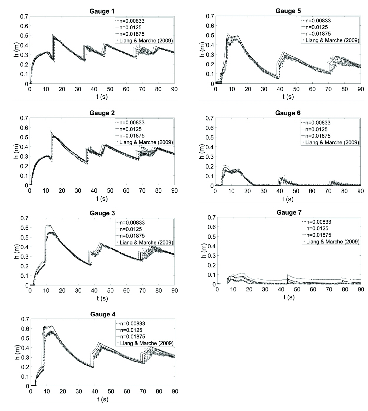
Time series of water depths at 7 gauges are recorded to describe these complicated phenomena and compared with the experimental data in Fig. 5. At the initial time, the dam suddenly broke and the initial water at the reservoir rushed onto the downstream like a flood on a plain. The waterfront reached the left slope, climbed over the peak of the hump (gauge 1 to 6) and further arrived at the other side of the horizontal bottom (gauge 7) around t = 5 s. Because of an interaction between the incoming waves and the reflecting waves from the side of the hump, a shock wave formed and propagated back to the upstream boundary. On the other side of the hump, a rarefaction wave occurred and moved to the downstream boundary, which caused increase of water depth at the right side of the hump (gauge 7). Around t = 25 s, the shock wave reached and reflected from the wall at the upstream boundary. After this reflection, the second wave propagated to the downstream. These complex processes continued until the momentum energy was damped due to bottom friction and water mass passed through the downstream boundary.
Overall, the numerical simulations show good agreements with the experimental data in term of both the propagation speed and water depth. In particular, at gauges 1 and 2, numerical results are close to the measured data until t = 90 s. At gauges 3 to 6, numerical results around the first peak of water depths are higher than the measured data. At gauge 7 which is at the other side of the hump, numerical results are always higher than the measured data. These discrepancies might happen because the numerical solutions of the shallow water equations were made based on the assumption of neglecting dispersive terms which would spread out several components with different speeds. If we simulate these flow phenomena using the Boussinesq equations which include dispersive terms, we would get solutions closer to the experimental data. When the Manning’s roughness coefficient n increases, the flow speed decreases at the first wave and the flow thickness increases at all the 7 gauges. Especially, at gauges 3 to 6, due to the adverse slope of the hump, with the increase of the Manning’s n, the flow thickness decreases at the first peak. The Manning’s n equal to 0.0125 gives the numerical solutions closest to the measured data.
3.2 Validation for debris flow
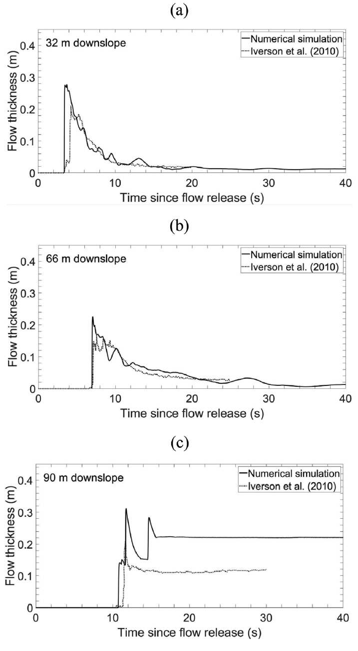
The present landslide model is applied for debris flow on the well-known large-scale USGS experimental flume. This experiment which was conducted on September 13, 2001 (Iverson, 2003; Iverson et al., 2010) has been investigated by several researchers to test their debris flow models (Denlinger and Iverson, 2001; Paik, 2015). The flume is a rectangular concrete channel, 95 m long, 2 m wide, and 1.2 m deep. The main part of the channel has a steep slope of 31o and is connected with a curve to the runout surface having a mild slope of 2.4o. The debris flow from the main channel would deposit at the 4 m wide runout surface. A volume of saturated soil has a mass of 9.4 m3 consisting of sand-gravelmud (SGM) material and is suddenly opened by a vertical headgate. More detailed information about the experimental facilities was reported in Iverson (2003) and Iverson et al. (2010).
Numerical simulation is conducted using the soil density of ρ = 2100 kg/m3, the Manning’s roughness coefficient of n = 0.034 m−1/3s, and the effective friction coefficient of μ = 0.12. The grid size is 0.1 m and the CFL number is 0.9 which guarantees numerical stability. During simulation we use a constant value of 2 m channel width because the numerical model is horizontally one dimensional. In the real experiment, however, the width changed from 2 m at the main channel to 4 m at the runout surface. This width change would cause numerical solutions different from the experimental data on the area of the runout surface.
Fig. 6 compares numerical results of debris flow thickness with measurement data at locations of x = 32 m, 66m, 90 m downstream of the headgate. It should be noticed that the location x is not the horizontal distance but the downslope distance on the bottom. The first and second locations are in the main channel while the third location is on the runout surface. Due to turbulent high speed of the debris flow on the steep channel, high fluctuation of the solutions occurred at the first and second locations in the present high-resolution numerical model. To smooth the highly fluctuating solutions, we use the moving average algorithm as given by
where yk is the raw (noisy) data, (yk)s is the smoothed data, the odd number 2n + 1 is named as the filter width or span. The greater the filter width is, the smoother the data are. In order to smooth these time series data of the flow thickness, we choose the value of span 2n + 1 = 101 which is equivalent to value of n = 50 and repeat smoothing process again. The results after smoothing are shown in Figs. 6(a) and 6(b).
On the whole, the numerical simulations are in good agreement with the experimental data, especially in term of the flow speed and flow thickness. Although the amplitudes are overestimated, the peakedness and the fluctuation of the computed results represent the effects of friction terms in the momentum equation. The peaks of the simulating results are higher than the measurement data due to the assumption of being hydrostatic in the shallow water equations as mentioned in the previous test. The time series data which are measured at x = 32 m and x = 66 m in Fig. 6(a) and Fig. 6(b), respectively, show better agreements than those at x = 90 m. These differences are of the curvature connected between bed slope of 31° and the flat bottom of 2.4° is not represented well in this simulation. Moreover, in the present 1D model, the width of the channel of 2 m is taken into account for the whole domain while that of runout surface of 4 m is set at this point of the experiment as mentioned previously. It results in the overestimation of approximate 50% in term of the flow thickness on the runout surface.
4. Model Application to Subaerial and Submarine Landslides
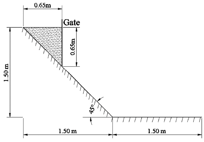
The debris flows over and under the water surface are called as the subaerial and submarine landslides, respectively. The subaerial landslide is affected by the subaerial gravity acceleration g0 = 9.81 m/s2 whereas the submarine landslide is affected by the buoyancy gravity acceleration g1 = g0(ρs − ρw/ρs where ρs and ρw are densities of soil and water, respectively. Rzadkiewicz et al. (1997) conducted hydraulic experiment of a submarine landslide and the induced tsunami. The volume of soil in a triangular section with 0.65 m × 0.65 m suddenly slid down on a slope of 45° which was connected to a horizontal bottom and the tsunami occurs due to the landslide. They also simulated the phenomenon using 2-dimensional (x, z) Navier-Stokes equations. In this study, we conduct numerical experiments of subaerial and submarine landslides using their model scales (see Fig. 7). However, we use different properties of ρ = 2100 kg/m3, n = 0.034 m−1/3s, μ = 0.08 following Paik (2015) who simulated landslides using the Saint-Venant equations. The grid size is Δx = 1 cm and the CFL number is 0.9 which guarantees a numerical stability.
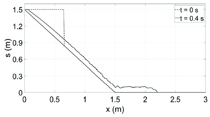
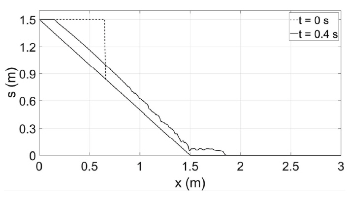
Figs. 8 and 9 show surface elevations of the subaerial and submarine landslides, respectively, at t = 0.4 s. For the submarine landslide, due to the buoyancy effect, the acceleration is reduced to g1 = 0.52g0 and the soils move more slowly compared to the subaerial landslide.
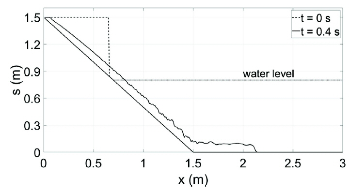
Fig. 10 shows surface elevations of combined subaerialsubmarine landslide at t = 0.4 s for the water surface at sw = 0.8 m. Subaerial landslide occurs above the water surface while submarine landslide occurs below the water surface. For the submarine landslide, due to the buoyancy effect, the acceleration is reduced to g1 = 0.52g0 and the soils move more slowly compared to the subaerial landslide. Therefore, for this combined subaerial-submarine landslide, the soils move more slowly compared to the subaerial landslide (Fig. 8). However, they move faster compared to the submarine landslide (Fig. 9).
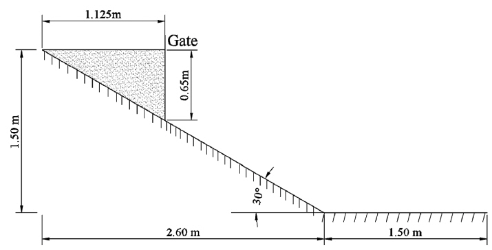
The next case study is to investigate the sensitivity of debris flow with different parameters. We change the angle of slopes from θ = 45° to θ = 30°. Fig. 11 shows the topography for simulating subaerial landslide with bottom slope of θ = 30°.
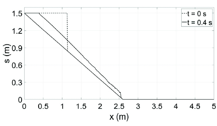
Fig. 12 shows the numerical solutions of surface elevations of subaerial landslide with bottom slope of θ = 30° at t = 0.4 s. After comparison with the solution with θ = 45° shown in Fig. 8, we find that the velocity increases with the increase of the bottom slope. These results are physically reasonable.
Furthermore, we compare numerical results with different Manning’s roughness coefficient of n = 0.034 m−1/3s and n = 0.051 m−1/3s which are different with a ratio of 1.5. It is clear that the propagation speed of the debris flow depends on the bottom roughness coefficient.
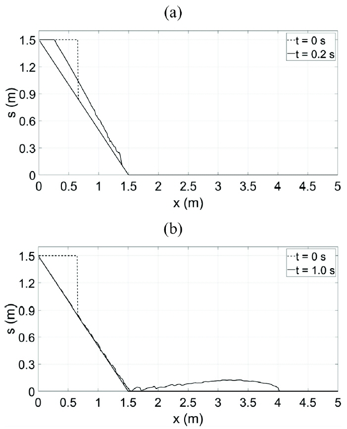
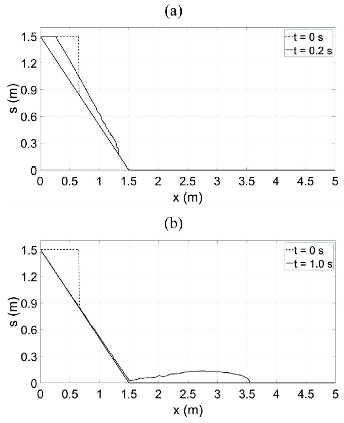
Figs. 13 and 14 show numerical solutions of surface elevations of subaerial landslide with Manning’s n of 0.034 m−1/3s and 0.051 m−1/3s, respectively. The speeds of landslides of the two cases are slightly different at t = 0.2 s, but the two speeds become more clearly different at t = 1.0 s. This implies that larger bottom roughness cause slower speed of the debris flow which was mentioned also by the previous works (Mikoš et al., 2006; Paik, 2015).
5. Conclusions
In this study, we investigated subaerial and submarine landslides using the finite volume scheme in the one-dimensional (x) shallow water equations. We used the (b, s) coordinate system to express the shallow water equations which can be applied in coastal zone as well as river. To discretize the governing equations, we used the well-known high-resolution scheme which combines the TVD limiter function and the second-order Godunov method (WAF method) employing HLL approximate Riemann solver. This scheme can deal with the wet/dry problems occurring in the real landslide phenomena. We applied both the conservative and alternative conservative forms of the shallow water equations to a dam-break water flow and found that the conservative form of the equations yielded accurate solutions in the dry/wet boundaries but the alternative conservative form yielded inaccurate solutions. We further verified the developed numerical model by comparing numerical results with the analytical solutions and the experimental measurements for both the dam-break water flow and the debris flow. We also applied the model to subaerial landslides with different bottom slopes and bottom frictions and found that both steeper bottom slope and smaller bottom friction cause faster movement of soils. In the future, the two-dimensional (x, y) shallow water equations as well as the non-hydrostatic equations (e.g., the Boussinesq equations) will be developed to accurately solve the subaerial and submarine landslide phenomena.