Sediment Particulate Motions Over a Ripple Under Different Wave Amplitude Conditions
파랑에 의한 해저 사련 위에서의 유사입자의 거동 특성
Article information
Abstract
Sediment particle motions have been numerically simulated over a sinusoidal ripple. Turbulent boundary layer flows are generated by Large Eddy Simulation, and the sediment particle motions are simulated using Lagrangian particle tracking method. Two unsteady flow conditions are used in the experiment by employing two different wave amplitudes while keeping other conditions such as wave period same. As expected, the amount of suspended sediment particles is clearly dependent on the wave amplitude as it is increasing with increasing flow intensity. However, it is also observed that the pattern of suspension may be different as well due to the only different condition caused by wave amplitude. Specially, the time of maximum sediment suspension within the wave period is not coincident between the two cases because sediment suspension is strongly affected by the existence of turbulent eddies that are formed at different times over the ripple between the two cases as well. The role of these turbulent eddies on sediment suspension is important as it is also confirmed in previous researches. However, it is also found the time of these eddies’ formation may also dependent on the wave amplitude over rippled beds. Therefore, it has been proved that various flow as well as geometric conditions under waves has to be considered in order to have better understanding on the sediment suspension process over ripples. In addition, it is found that high turbulent energy and strong upward flow velocities occur during the time of eddy formation, which also supports high suspension rate at these time steps. The results indicate that the relationship between the structure of flows and bedforms has to be carefully examined in studying sediment suspension at coastal regions.
Trans Abstract
부유 퇴적물의 입자 운동에 대한 수치실험이 굴곡이 있는 해저면 위에서 수행되었다. 해저면 경계층의 난류 유속장은 LES 난류모델을 사용하여 구현하였고, 난류 흐름 속에서의 퇴적물 입자운동은 Lagrangian 입자추적 모델을 사용하여 구현하였다. 수치실험을 통하여 두개의 다른 유속조건을 사용하였는데, 파랑주기를 비롯한 다른 모든 조건은 동일하게 유지한 가운데 오직 최대 유속만 다르게 하여 실험을 수행하였다. 예상한 것과 같이 부유되는 퇴적물 입자의 양은 유속이 강할 수록 증가하였다. 그러나 예상하지 못한 결과도 관측되었는데 그것은 비록 최대유속 외에 다른 모든 조건은 동일하더라도 퇴적물이 부유되는 양상은 다르게 나타날 수 있다는 것이다. 특히 퇴적물이 부유하게 되는 시간이 위상평균한 파장 주기안에서 서로 다르게 나타나는 것이 발견되었는데, 이는 해저면 굴곡 주위에서 유속에 의해 생성되는 난류 와동의 생성시간이 다르기 때문에 일어나는 것으로 밝혀졌다. 이전의 연구에서도 알려진 바와 같이 이런 난류 와동들이 퇴적물의 부유현상에 미치는 영향은 지대한 것으로 확인되었으며, 또한 이런 와동들의 생성시간은 유속의 크기에 따라 달라 질 수 있음이 밝혀졌다. 이로인해 해저면 굴곡 위에서 퇴적물의 부유현상을 보다 정확하게 규명하기 위해서는 파랑의 여러가지 복잡한 변수들을 고려하여야 함이 이번 실험을 통하여 입증되었다. 또한 퇴적물 입자의 부유에 영향을 미치는 난류 에너지분포 역시 생성된 난류 와동에 많은 영향을 받는 것으로 나타났다. 이번 연구를 통하여 유속의 세기변화 만으로도 퇴적물이 부유되는 시간이 굴곡이 있는 해저면에서 바뀔 수 있는 것으로 확인되었으며, 이는 향후 퇴적물 부유에 대한 연구를 할때 해저면 구조와 유속구조의 상관관계를 보다 신중히 검토해야 함이 밝혀졌다.
1. Introduction
Sediment suspension in nearshore regions is caused by combined action of waves and currents, and it is important to understand the process in order to predict sediment transport or to protect coastlines from erosions/depositions in that area.
However, it is a very complicated process not only because the breaking shallow water waves are highly turbulent but also because seabeds are covered by various bedforms. First, the near-bed turbulent bottom boundary layer flows are difficult to understand due to the unsteadiness under coastal waves and currents. Moreover, various shaped seabed bedforms add complexity to the flow turbulence caused by eddies generated around these bedforms. These turbulent eddies play important role in sediment suspension because suspension process can be enhanced by picking-up and entrainment of sediment grains into these eddies from the seabeds. Recognizing this importance, the study of turbulent eddies and their relationship with sediment suspension process are crucial in understanding sediment transport in coastal regions. It is because the formation of these eddies can determine when and where are the sediments suspended over seabeds, and therefore the total amounts and overall directions of sediment motions in that area are highly dependent on this special pattern of suspension process.
Various conceptual models have been suggested for the sediment suspension pattern over rippled seabeds by early investigators (Bagnold, 1946; Bagnold, 1966; Nielsen, 1979; Sleath, 1984; Fredsoe and Deigaard, 1992; Nielsen, 1992).
The role of turbulent eddies formed in the lee of the ripple crest (lee eddies) in capturing and sediment particles were studied in these models in which these sediment-carrying eddies are ejected and carried away with suspended sediments as flows are reversed. Since these conceptual models on the role of lee eddy on sediment suspension are not easily examined by in situ or lab experiments, various numerical models have been studied over rippled and flat beds (e.g. Hansen et al., 1994; Zedler and Street, 2001; Vittori, 2003).
In our previous studies, we also have performed various numerically studies on sediment suspension over flat and rippled beds under steady as well as unsteady turbulent bottom boundary layer flow conditions. First, by combining a Reynolds Averaged Navier-Stokes equation model(RANS) with sediment advection-diffusion equation (Tjerry, 1995; Andersen, 1999), a field observed suspended sediment concentration(SSC) data were compared with model results, showing that the amount SSC by the model was underestimated although the pattern of sediment suspension was successfully recovered by the model during the phaseaveraged wave period over long wave ripples (Chang and Hanes, 2004). As RANS is less accurate in generating turbulent flow energy over rippled bed than Large eddy Simulation (LES) (Chang and Scoti, 2004), a LES model has been employed to generate turbulent boundary layer flow field by combining Maxey and Riley equation (1983) to simulate particulate motions of suspended sediment particles. When the sediment motions were examined over a sinusoidal ripple in a steady flow (Chang and Scotti, 2003), streaky coherent vortices were developed over the ripple crest in the streamwise direction and they captured and carried sediment particles over the crest. These sediments carried within coherent vortices were then ejected into the lee area of the crest, enhancing sediment suspension in this area. Sediment particle motions in turbulent boundary layers were also investigated under an unsteady flow condition but over a flat bed (Chang and Scotti, 2006). During the maximum flow rate, similar coherent streamwise turbulent vortices were developed to carry sediment particles in the same flow direction close to the bottom. During the flow reversal, however, turbulent vortices were developed vertically and they actively dispersed sediment particles in the vertical direction, producing strong suspension events at this time. This is an important result as it is incompatible with simple eddy ‘diffusion’ type sediment suspension models, but suggesting high possibility of significant role of sediment ‘convection’ by flow turbulent structures in the process of sediment suspension under waves. Recently, Chang et al. (2013a) reported statistical results on the sediment suspension under wave conditions by confirming the consistent pattern of sediment suspension over flat bed, emphasizing the importance of flow reversals on the suspension event. Over rippled bed, however, there are significant difference were found in the sediment suspension pattern under unsteady flow conditions (Chang et al., 2013b). In this case, a turbulent lee eddy was generated during the maximum flow rate and the decelerating wave phase, and the sediment suspension becomes active and strong due to the turbulent vortical structures caused by this lee eddy. Therefore, the strongest sediment suspension event during the time of flow reversal over flat bed was not found over a rippled bed. Instead, a significant phase shift was found in the suspension process. In order to examine the consistency of this phase shift in sediment suspension over rippled seabeds, another experiment was implemented with similar numerical setting with Chang et al. (2013b) but by changing the flow conditions using different wave periods (Chang et al., 2013c). As a result, the phase shifts in the time of maximum sediment suspension were even found between the waves with different periods because the time of lee eddy formation is changed with varying wave periods. This result may lead to significant changes in understanding of sediment suspension process because this process has been generally understood in terms of the averaged wave phase regardless of their periods. If the suspension pattern has phase shifts between waves with different period, however, the phase-averaged method to describe suspension pattern over ripples would not be valid anymore.
In the present study, we extend the previous researches by performing another experiment to enhance the understanding of the relationship between the flow condition and sediment suspension pattern. For this, two different flow conditions are additionally employed by changing the flow strength but keeping the other flow conditions such as wave periods same. The purpose of present study is then to examine any possible variation or anomaly in sediment suspension events from the conventional framework of understanding of suspension process with this minimal change of flow conditions.
2. Numerical Experiment
Numerical setting of present experiment is basically same with previous studies (Chang et al., 2013b; Chang et al., 2013c) with the only difference through changing the flow strength. So, readers are recommended to consult these previous articles for more details of model descriptions, and only briefly described here.
The near-bed boundary layer flow and pressure fields are calculated by LES solving a filtered Navier-Stokes equations
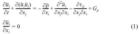
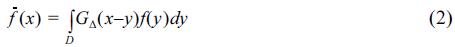
where the filtered variable is given by
In Eqn, (1), the subgrid-scale stress is modeled using dynamic eddy viscosity (Meneveau et al., 1996).

The unsteady wave condition is generated using an external forcing using pressure gradient.

In Eqn. (4), the steady component and oscillating wave amplitude are given by controlling Gsp and Gop respectively.
In the present study, these parameters are controlled to have two different wave amplitudes (amplitude of wave velocity outside the boundary layer), U0, as 0.13 m/sec and 0.26 m/sec. The oscillating wave period, T, which is controlled by Ω in Eqn. (4), is set to 2 seconds for the present experiment. This short wave period is especially employed in order to increase flow turbulent energy due to short intervals between the two flow reversals (Chang et al., 2013c).
The computational domain is a channel with wavy bottom that creates the effect of sinusoidal ripple by applying no-slip condition on the ripple surface using an immersed boundary technique (Fadlun et al., 2000). The channel height is 5 cm, and streamwise (x direction) and spanwise (y direction) channel widths are 10 cm respectively. The equally spaced grid points are 290 in the streamwise direction and 66 points in the spanwise direction. Vertically, total 130 grid points are set to have more fine grids near the ripple. The ripple length and height are set to 5cm and 5 mm respectively (Fig. 1).
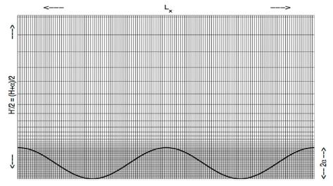
Side view of the computational geometry with grids (Chang et al., 2013b).
Lagrangian model for sediment particle motions in the turbulent boundary layer flows are calculating the Maxey and Riley(1983)’s equation by ejecting each particles with incipient velocity from the surface of the ripple as described in Wiberg and Smith (1985),
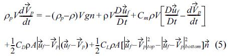
where the velocity of individual sediment particles, VP, is calculated from the balance between buoyancy, flow pressure, added mass, drag and lift forces. Once VP is calculated from Eqn. (5), the position of each sediment particle, xP is calculated in the Lagrangian framework, dxP/dt = VP. Initially, 6000 sediment particles with diameter, D = 10 μm, are located on the ripple surface. The density of sediment grains is set to 2.65 as it is set to same density as quartz. Once the local shear stress exceeds a threshold that is determined by Celik and Rodi (1991), the sediment particles are injected into the turbulent flows with initial velocity given in Chang and Scotti (2003).
3. Results
As described earlier, two different flow conditions in the present study are generated by controlling the two parameters, Gsp and Gop in Eqn. (4). For Case 1, wave amplitudes, U0 is set to 0.13 m/sec and U0 is set to 0.26 m/sec for Case 2. Fig. 2 compares the two streamwise mean (phase averaged) flow velocities over one wave period. The flow velocities are measured at x = 5 cm and z = 7 mm which is the location of 2 mm over the center of ripple crest where the motions of sediment particles are directly influenced by these local flows. As shown in Fig. 2, the main difference between the two flow conditions is the magnitude of maximum flow velocities. While the maximum velocity magnitude is about 0.2 m/sec for case 1, the magnitude is about 0.35 m/sec for Case 2. These maximum velocity magnitudes are lager than the oscillating wave amplitude, U0, for both cases due to the steady component, Gsp, in Eqn. (4). Gsp is controlled respectively for each cases in order to make the mean local flows to be comparable between the two cases except for the flow intensity as shown in Fig. 2. In addition, it is necessary to have mean flow components as it is commonly found in the real waves in the coastal regions, which adds complexity in understanding turbulent bottom boundary layer flows due to the flow asymmetry. Except for the difference in velocity magnitudes, all other flow and geometry conditions are kept same between the two cases. Also, although the time of flow reversals are not identical, the overall flow pattern is similar between the two cases. Therefore, it is reasonable that we aim to examine sediment suspension process through comparison between two different flow strength conditions from the experimental set up of present study.
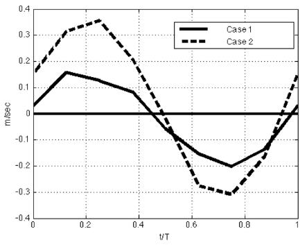
Streamwise velocities phase averaged over one wave period at 2 mm over the ripple crest. (solid: U0 = 0.13m/s (Case 1), dashed: U0 = 0.26 m/s (Case 2)).
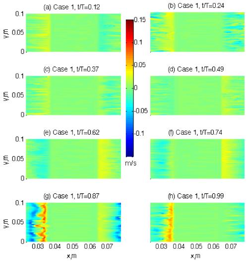
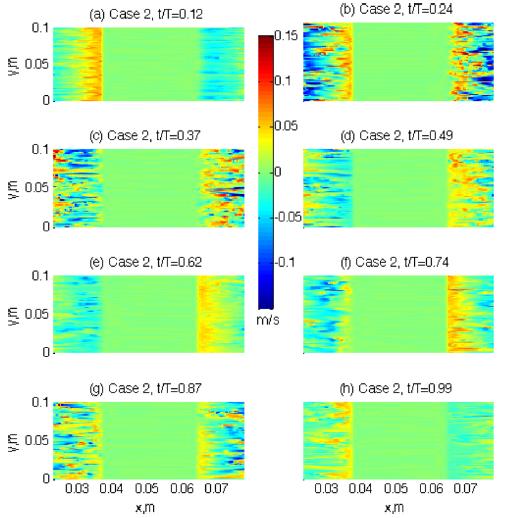
The flow pattern around the ripple is compared between the two cases in Fig. 3 and 4. Two dimensional (‘x-z’ plane) flow vectors are calculated at eight different time steps by averaging the flows in the spanwise (y -) direction. The eight time steps are chosen to show each wave phase according to the freestream velocities (outside the boundary layer). So, t/T = 0.12 in panel (a) is the ‘accelerating flow phase’ and t/T = 0.24 in panel (b) is the ‘maximum flow rate’ according to the freestream flow phases, while t/T = 0.37 and 0.49 in panel (c) and (d) are the ‘decelerating flow phase’ and ‘the time of flow reversal’ respectively. When compared with the flow pattern in Fig. 2, these eight wave phases of the freestream are generally agreed with local flow phases near the ripple crest. The other four time steps from t/T = 0.62 to 0.99 in panels from (e) to (h) are the repeating of the preceding four wave phases but in the reversed flows. As clearly shown in both figures, the flow strengths are greater in Case 2 than Case 1 as it is expected from mean flow pattern in Fig. 2. However, there is a significant difference in the flow pattern around the ripple between the two cases. The turbulent eddies are formed in the lee area of the ripple crest, and the time of these eddy formation is different between the two cases.
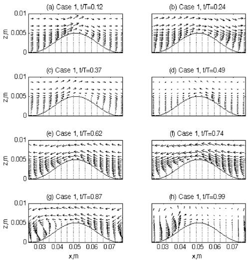
Velocity vectors around the ripple at eight different time steps for Case 1 (U0 = 0.13 m/s). Velocity vectors in all panels are drawn in same scale.
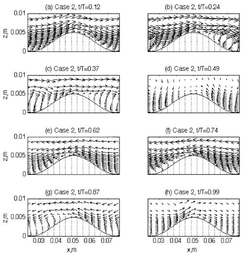
Same with Fig. 3 but for Case 2 (U0 = 0.26 m/s). Velocity vectors are drawn in same scale with Fig. 3 for direct comparison.
The lee eddies are formed when flows are separated in the lee side of the crest. However, these lee eddies are not always formed around ripples because it also depends on the size of the ripple. Bagnold (1946) first classified ripples into two types: rolling-grain ripples and vortex ripples. The rolling-grain ripples have so small height that no real eddy formation takes place in the lee area of the ripple (Fredsoe and Deigaard, 1992). The vortex ripples are higher and steeper so that this maximum slope close to the avalanche angle is assumed to be responsible for flow separation behind the crest, which induces the vortex formation (Rousseaux et al., 2004). In their Lab experiment, Rousseaux et al. (2004) observed that eddies could be even formed over rolling-grain ripples too. In their experiment, they suggested two non-dimensional parameters to determine the ripple regime; ε = h/2δ, and r = 2A/λ where h is ripple height,  is the Stokes layer thickness with kinematic viscosity, v, and oscillating frequency, f. Also, r is defined with fluid particle displacement, 2A, and ripple wavelength λ. Usually the rolling-grain ripples are defined at low values of both numbers, ε < 1 and r < 1. In the present experiment, both of the parameters are higher than 1 as ε ~ 6 and r ~ 1 − 2 . So, the ripple of the present study belongs to the range of vortex ripple, and so lee eddies are expected to form. Even over the vortex ripples, however, the pattern of the lee eddies and the conditions to form them are not easily predictable, and even difficult to observe them. Barr et al. (2004) solved time-dependent Navier-Stokes equations. Using curvilinear grid system, they tested different shapes of ripples (but with similar dimensions) to examine their impact on the flow fields. They found that flow separation from the ripple crest is a mechanism for the production of turbulence in the boundary layer during phases of maximum flow and has been associated with turbulent boundary layer growth over steep ripples. As the steepness of the ripples increases, the turbulence becomes more focused in the trough and above the ripple crest, which may imply smaller chance of lee eddy formation in case of steeper ripples. In addition, Zedler and Street (2001) used a LES to investigate steady flow structures over various three-dimensional ripples. Although they did not apply unsteady flow conditions in their experiments, the features of lee eddies and their role in transporting suspended sediments widely varied according to the ripple shapes along with the generated near-bed eddy cores that captured sediments within it. The role of lee eddies and various sized vortex ripples are also tested by lab experiments (Scherer et al., 1999). In this experiment, the formation and advection of lee eddies over various sized vortex ripples were investigated by changing unsteady flow conditions such as wave frequency and sediment grain size. The results showed that the size and shape of lee eddies and their appearance/disappearance related to their movement have very complicated relationship between the flow conditions and ripple dimensions. Therefore, the prediction of lee eddy formation over a ripple is not an easy mechanism. Although the ripple dimension is the one of the most important factors to develop lee eddies, turbulent boundary layer flow structure also plays important role in the mechanism to form lee eddies. For example, Andersen(1999) suggested a Reynolds number based on wave amplitude, ReA = AU0/v is an important parameter for the dynamics of vortex ripples and for the formation of lee eddies with higher chance of lee eddies with increasing A. Blondeaux and Vittori (1991) analyzed dynamics of lee eddies by solving vorticity equation and the Poisson equation. According to their results, there are two contributions of the flows around ripples to form vortices − one periodic in time and the other time independent steady part. The steady part may form recirculating cells along the ripple slope. These recirculating cells consist of two closed streamlines in the lee area of the ripple crest, leading to flow separation and so possibly forming a lee eddy. The size, location, and movement of this lee eddy caused by the steady part are also dependent on the ripple as well as flow conditions. Another contribution to form a lee vortex around ripple is the oscillating part. With their experimental set up, positive vorticity generates along the profile near the crest in the accelerating flow phase. As time advances, boundary layer along the downstream gets thickened and vorticity with opposite sign is generated at the bottom until the flow is separated. Then, the rolling up of positive vorticity created a vortex structure – forming lee eddy. Therefore, one of the most important conditions to form a lee eddy over rippled bed is the flow separation either it is by steady component or by flow oscillation. However, even the flow separation is not easily understood as it is a complicated combination between the ripple and flow conditions as well. In addition, if the flows are not purely oscillating waves but pulsating structures as it is commonly found in the real fields and as it is in our cases, the combined wave and current flow structure would add complexity to the mechanism of the formation and motion of the eddies around ripples (Andersen, 1999).
These complicated process to form lee eddies are well reflected in the present experiment. As shown in Fig. 3 and 4, the lee eddies are formed at different flow phase although the ripple dimension is same between the two cases. Although flow separation commonly start at the accelerating phase or the maximum flow rate over vortex ripples, no separation are found in Case 1 at these flow phases (t/T = 0.12 and 0.24). In Case 2, it shows more general pattern of flow separation. As the flow accelerates (t/T = 0.12), near-bed flows along the downslope starts to be directed opposite direction, leading to flow separation. This flow separation develops into a lee eddy at the time of maximum flow rate (t/T = 0.24). This lee eddy rapidly grows in strength and becomes maximum in size at the time of flow deceleration (t/T = 0.37) before the flow reversed. For Case 1, however, this process of lee eddy formation is not seen during the first half of the wave cycle. This failure in forming a lee eddy is probably due to the lower flow strength, which leads to lower Reynolds number, ReA at this wave phase. After flows are reversed, however, flows are separated at t/T = 0.74 and a lee eddy is formed at the decelerating flow phase (t/T = 0.87). As reviewed earlier, it is not easy to explain why there is difference in the time of eddy formation during one wave cycle because many factors are involved and they are likely interrelated too. However, one possibility can be found from Fig. 2. As already mentioned, the flows in the present study have asymmetries due to the steady component Gsp in Eqn. (4), and the maximum magnitudes of flow velocities during each half wave cycle are different in each case.
For example, the maximum velocity magnitude during the first half wave cycle is about 0.16 m/sec for Case 1(Fig. 2). However, the maximum velocity magnitude during the latter half cycle is about 0.20 m/sec. Although this difference in velocity magnitude looks small, this small change can make big difference in eddy formation as is shown in Fig. 3. Similarly, the velocity magnitude is also different in Case 2 as well. Although the maximum velocity magnitude during the first wave cycle is about 0.35 m/sec, the magnitude during the latter cycle is only about 0.30 m/sec. Again, the difference between these velocity magnitudes is not significant. However, the lee eddies formed during both of the wave cycles are much different in size and strength. While the lee eddy formed during the first wave cycle is conspicuous, the eddy in the latter cycle is much weaker and even not clearly visualized with the velocity vectors (t/T = 0.87).
This difference in time of eddy formation between the two cases can make difference in the pattern of sediment suspension as well. Fig. 5 and 6 compare the sediment particle distributions over the ripple at first eight time steps after they were launched. These eight time steps are not identical to the time steps of the flow vectors in Figs. 3 and 4, but close enough to have direct comparison between the flow patterns and sediment distributions. As it is clearly seen from the figures, the amounts of suspended sediment particles are distinguished between the two cases. Specially, it is interesting to find that only a few sediment particles are suspended from the ripple surface during first half of the wave cycle for Case 1. During the accelerating phase (Panels (a), Fig. 5), some of particles are pushed upslope until they reach the crest. After that, these particles are ejected into the lee area of the crest during the maximum flow rate (Panel (b)). This motion of particles corresponds to the sediment carrying process described in the previous study (Chang and Scotti, 2003), in which steady flows around the ripple produced long streaky coherent vortex pairs along the upslope of the ripple in the streamwise direction. These streaky coherent vortices then captured sediment particles within them, and carried up to the ripple crest. The sediments that were carried by these coherent cortices were ejected into the lee area after they reached the crest. Although those coherent structures are not visualized in the present study, the pattern of sediment movement shown in Panels (a) and (b) in Fig. 5 is very similar to the previous steady case as sediment particles that initially lie on the upslope of the ripple are pushed up to the crest as likely being captured by the streaky coherent vortices, and ejected into the lee area during the maximum flow phase. However, the process to carry sediments upslope along the ripple surface does not seem to be followed by active sediment suspension process in the lee area of the crest. Not only too small numbers of sediments are moving during this wave phases, but also there is no clear vertical dispersion on the sediments that are ejected into the lee area. Although there are some sediment particles that are pushed upslope until they reach the top of crest and then ejected into the lee area, those sediments do not have active vertical dispersion during the time of decelerating flow phase (Panel (c) in Fig. 5).
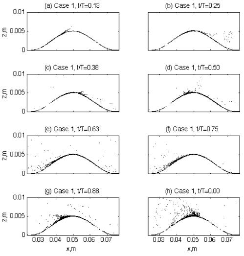
Sediment particle distribution around the ripple at the first eight different time steps since particles are initially launched (Case 1). The time steps are not identical but clos enough to the eight time steps in Fig. 3 and 4.
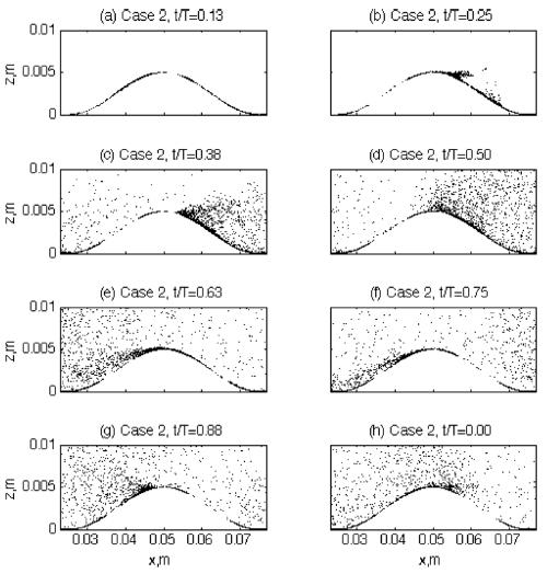
Same with Fig. 5 but Case 2.
In Case 2, however, the sediment suspension pattern is much different from Case 1 during the first half of the wave cycle. At the maximum flow rate (Panel (b)), sediment particles are ejected from the ripple crest into the lee area, which is similar to Case 1. However, a bunch of particles are suspended from the bottom of the downslope of the ripple. This suspension event occurring at the ripple downslope is caused by the action of lee eddy shown in panel (b) in Fig. 4. If the two panel (b)s in Figs. 4 and 6 are compared, it is not difficult to relate the eddy pattern with sediment motions as the sediments are likely being entrained into the lee eddy from the bottom. Since the direction of the near-bed flow along the downslope is in the opposite direction to the streamwise mean outer flows due to the lee eddy, the sediment particles that are suspended from the bottom of downslope is also in the counter-streamwise direction. In addition, lots of sediment particles are dispersed vertically during the decelerating flow phase (Panel (c) in Fig. 6). Due to this strong dispersion process, some particles even reach up to the outer flow region (~0.01 m). This high rate of sediment suspension and strong vertical dispersion of particles at this decelerating wave phase is also caused by the strong lee eddy motion (compare with panel (c) in Fig. 4). More details on the relationship between the lee eddy and the vertical dispersion will be discussed later. Based on the description from the Figs. from 3 to 6, however, the strong sediment suspension events are at least closely related to the eddies formed in the lee area as further evidence for this can be found from Case 1 during the latter half wave cycle. When there is no lee eddy formed during the first half cycle, sediment suspension is poor and negligible. During the latter half cycle, however, there is an eddy formed at the deceleration phase at t/T = 0.87 (Panel (g) in Fig. 3) and later, this eddy motion produces strong counter flows upslope the ripple at t/T = 0.99 (Panel (h)). If this turbulent flow pattern caused by lee eddy is compared with the sediment suspension pattern in panel (g) and (h) in Fig. 5, it is found that more sediment particles are suspended from the bottom of the ripple downslope by the eddy, and they are hurled up into the outer flows due to stronger vertical dispersion than the first half wave cycle. Therefore, although the pattern of sediment suspension is out of phase between the two cases because of the different time of maximum suspension event, this difference is also caused by the formation of lee eddy. That is, the sediment suspension process is reinforced by the lee eddies over rippled beds - while the amount of suspended sediments is strongly related to the strength of the mean flows, it is the lee eddies that directly affects the time of the strongest suspension event in the wave cycle. The timing of suspension events is one of the most important factors in studying sediment transport in coastal regions. For example, if the maximum suspension occurs during the incoming half wave cycle, total sediment transport would be directed onshore. If the suspension is stronger during the outgoing wave cycle, however, sediments would be moved into offshore.
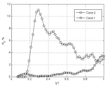
The time of sediment suspension events is also investigated by estimating sediment suspension rate. In Fig. 7, the sediment suspension rate, Rt, is calculated for the comparison. Usually, it is not easy to determine the rate of suspension due to the difficulty to define ‘suspension’ from the choice of reference level and concentration. In our previous studies (Chang et al., 2013c), a new measure to estimate suspension rate was developed. In this measure, the suspension rate, Rt, is defined as a ratio between the number of sediment particles that remain close the bottom and that leave the bottom area as it is defined if the distance from the ripple surface is greater than a certain limit. Based on this description, Rt is defines as
Sediment suspension rate, Rt.

where n(Pa) is the number of particles whose distance from the bed,  , is less than a limit, lt, at a reference time step t1, and n(Pb) is the number of particles out of Pa that leave the surface area (i.e. l > lt) at some time later, t = t1 + Δt. In the present experiment, lt is set to 0.5 mm, and Δt is set to 0.2 sec. The sediment particles are initially distributed evenly at the surface of the ripple. Although this measure is not a perfect measure to estimate the rate of sediment suspension, it is still useful to understand the suspension pattern within the frame of one wave phase.
Fig. 7 compares Rt between the two cases. As it is expected from the descriptions of previous figures, the suspension rate is much higher in Case 2 than Case 1. However, the peak time of Rt of both cases gives some significant information. For Case 1, the suspension rate is low for the most time of the wave cycle. But it sharply increases after t/T ~ 0.8. If reminded by the fact that the lee eddy is formed at t/T = 0.87 and its role in sediment suspension, this increase of Rt at this time is due to the motion of lee eddy formed at this time. Also in Case 2, although Rt is greater than Case 1 for the most of the time, it decreases after it is peaked at t/T~0.3. Since the lee eddy was strongly developed at t/T = 0.24 and 0.37 in Fig. 4, this peak in suspension rate in Case 2 is also caused by the lee eddy motion.
Another measure to examine the relationship between lee eddy and sediment suspension is the turbulent energy distribution. As Chang and Scotti (2004) pointed out, modeling turbulent energy such as Reynolds stresses is a crucial factor in estimating sediment suspension. In the description of suspended sediment distribution using diffusion-advection model by solving suspended sediment concentration, C, the total sediment flux is given as

where W is vertical velocity, ws is sediment setting velocity, and vt is eddy diffusivity of suspended sediment concentration. Since Eqn. (7) is given through the Reynolds decomposition, the eddy diffusivity, vt, is given as a function of Reynolds stresses such as  and
and  . Due to the fact that sediment suspension is mainly related to the vertical motions of sediments, is one of the most important controlling factors to determine eddy diffusivity in Eqn. (7) and so, it is a very important component of turbulent energy that contributes to the suspension process. Figs. 8 and 9 compare the distribution of Reynolds stress at the same eight time steps with Figs. 3 and 4 between the two cases.
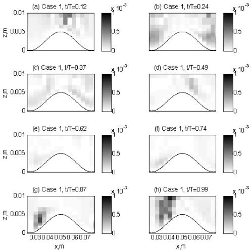
Reynolds stress () distribution around the ripple at the same eight time steps with Fig. 3 and 4. Case 1.
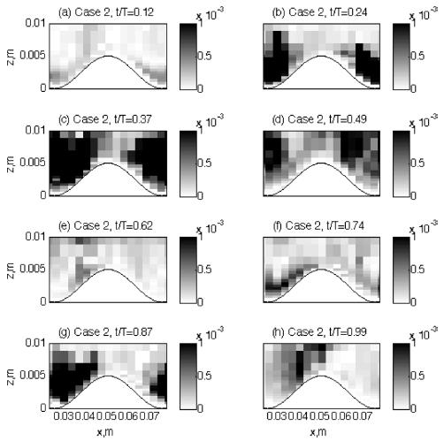
Same with Fig. 8 but for Case 2.
As it is expected, the magnitude of is much higher in Case 2 than Case 1, which means turbulent energy (specially vertical flux of turbulent energy) is much higher in Case 2. Also, due to the contribution of to the eddy diffusivity and also to the sediment suspension as given in Eqn. (7), The turbulent energy to support suspension events is much higher in Case 2 as well. Except for this consistency in the energy level of Reynolds stresses in relation to the amount of suspended sediment, the timing of distribution is also consistent with previous descriptions as the time of high level of is closely related to the time of eddy formation. In Case 1, although turbulent energy is low for the most of the time, higher values of are found at t/T = 0.87 and 0.99 which corresponds to the time of lee eddy formation. Even the locations of high values of correspond to the locations of lee eddies in panels (g) and (h) in Fig. 3. In Case 2, highest values of are found at t/T = 0.37 which is the time of maximum development of the lee eddy too. Based on the description of Figs. from 8 and 9, therefore, it is clear that turbulent energy increases due to the motion of the lee eddies, and so the enhancement in sediment suspension at the corresponding time steps is closely related to the eddy motions as well.
Another measure that can examine the effect of lee eddies on the sediment suspension is the distribution of the vertical component of flow velocities. In Figs. 10 and 11, the vertical velocities are projected on a horizontal plane (X-Y plane) at the elevation z = 2.5 mm. This elevation is half height of the ripple crest, so this horizontal plane shows the vertical velocity field of the lee side of the ripple where the motion of lee eddies and the suspension events are strongest.
Vertical component of flow velocities in X-Y horizontal plane and at elevation z = 2.5 mm. The velocities are measured at the same eight time steps with Fig. 3 and 4, Case 1.
Same with Fig. 10 but for Case 2.
For Case 1, the magnitude of vertical velocities is low at most of the time steps except t/T = 0.87 when is the time of the lee eddy formation. Not only the velocity magnitude is significantly at this time, but also the velocity distribution shows an interesting structure. While the upward velocities are found close to the crest, downward motions are found in the area further from the crest. This structure is also consistent with the flow pattern that is caused by the circulation of the lee eddy. Since the lee eddy has counterclockwise circulation at this time step (Panel (g) in Fig. 3), the vertical velocity field in Fig. 10 responds to the eddy motion with strong up and down velocities in the lee area. These strong vertical velocity components due to lee eddies are again closely related to the strong suspension events as sediment particles could disperse fast with these strong up and downward velocity components
The vertical velocity structure is more complicated in Case 2. Similarly to Case 1, general flow pattern corresponds to the motions of the lee eddy in Fig. 4 as strong up and down flow velocities are found consistently with the development of the lee eddy. However, the velocity structure is more turbulent compared to Case 1. For example, at t/T = 0.37 when the eddy motion is most active, the up and downward flow velocities show more disorganized structure than Case 1 (compare with panel (g) in Fig. 10). While the up and downward velocity pattern in Case 1 is more organized and it corresponds to the direction of eddy motion, the velocity components in opposite directions are mixed in the lee area in Case 2, having lots of hot spots of up and down velocities. This spotty structure of vertical velocity is caused by cloud of turbulent vortical structures as previously studied by Chang et al. (2013b). As the mean flow strength increases in Case 2, the Reynolds number, ReA, increases, and the flow becomes more turbulent, resulting in stronger development of turbulent structures.
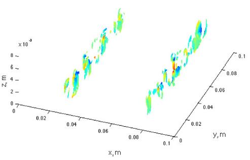
One way to visualize these turbulent structures is contouring the isosurfaces of second invariant of ∇u (Hunt et al., 1988).

where S and Ω are the symmetric and anti-symmetric component of ∇u. In Fig. 12, the isosurfaces of Q at t/T = 0.87 are contoured for Case1 while the isosurfaces of Q at t/T = 0.37 are contoured in Fig. 13 for Case 2. As can be seen from these figures, vortical turbulent structures are developed in the vertical direction in the lee area of the crest for both of the cases. The amounts of structures are, however, much less in Case 1 compared to Case 2. The two time steps, t/T = 0.87 and 0.37 for each case is chosen when the development of these turbulent structures are most active due to the lee eddy motions. Thus, the difference in the amount of turbulent cortical structures between the two cases is likely caused by the difference in the mean flow strength.
Isosurfaces of Q = 4000 at t/T = 0.87, Case 1. Isosurfaces are colored based on the local values of streamwise component of vorticity.

Same with Fig. 12 but t/T = 0.37 of Case 2.
Chang et al. (2013b) reviewed the significant role of these turbulent vortices in suspension of sediments. Many of the sediment particles that are ejected from the bottom are captured by these vertical vortices and also transported through them. Therefore, strong vertical sediment dispersion can occur by these turbulent vortical structures. The development of these turbulent structures is supported by the lee eddies because the flows near eddy become more turbulent due to the rotational motion of the eddy. However, the strength of these structures is also dependent on the mean flow strength as is seen by the difference in the amount of turbulent vortices between the two cases.
4. Conclusion
Events of sediment suspension are compared between two flow conditions with different flow strength. As previously studied, sediment suspension over rippled beds is a highly complicated process showing strong variability depending on the ripple geometry as well as flow conditions. For example, there was significant difference in the phase of suspension events between over flat and rippled beds (Chang et al. 2013b). In addition, even with all other conditions kept same, phase difference in suspension is still found between waves with different periods (Chang et al. 2013c). In the present study, we additionally aim to discover any unexpected changes in the suspension pattern under different flow conditions. Usually, it is expected that the time of sediment suspension would not change within the wave period if flow strength is the only conditional change (i.e. all other conditions are kept same). The results show, however, that not only the amount of suspended sediments but also the time of suspension events are changed due to the variation in flow strength. It occurs because the structure of flow turbulence is dependent on the mean flow velocities around ripples. When unsteady bottom boundary layer flow field is affected by the existence of bed ripples, the turbulence structure would become more complicated due to the effect of complex relationship between the flow and ripple conditions. Therefore, even under same geometric conditions, turbulent energy distribution can be changed in time and space due to small changes in flow conditions, or vice versa. As an example, the result of present study shows that the time of lee eddy formation is changed due to the change in flow strength. It is because the asymmetric velocity magnitudes caused by combined effect of steady and oscillating wave components can affect the formation of these lee eddies. The importance of these lee eddies in sediment suspension cannot be ignored because separation of flows can increase the turbulent flow energy especially the vertical component of Reynolds stresses. The result also shows that sediment suspension is greatly dependent on the eddy formation as suspension gets strengthened when and where are these lee eddies formed. This is an important finding because the pattern of suspension event such as timing of maximum suspension is possibly changed by only changing flow strength. Changes in wave phase of sediment suspension due to flow strength may lead to significant changes in estimating total sediment transport in the coastal regions. It is because different time of sediment suspension within wave period can lead to different cross-sectional directions of the total movement of suspended sediments. Meanwhile, the amount of suspended sediments under the motion of lee eddies still strongly depends on the mean flow strength regardless of the timing of suspension events. Considering the role of turbulent vortical structures that vertically develop in the lee area on the sediment suspension process, and also considering the difference in the amount of these structures due to flow conditions, it is the flow intensity that determines the amount of suspended sediments due to lee eddy motions. Present study has focused on the suspension events related to changes in flow conditions only. Therefore, it is recommended to extend the research with possible changes in ripple geometry in order to build up related parameters for future studies.
Acknowledgements
This work is funded by the Brain Pool Program from the Korea Federation of Science and Technology Societies, and by the projects “Development of Technology for CO2 Marine Geological Storage, “Development of Korea Operational Oceanographic System (KOOS), and “Kyeongbuk Sea Grant Program” from the Ministry of Oceans and Fisheries, Korea.