Statistical Characteristics of Hourly Tidal Levels around the Korean Peninsula
한반도 연안 1시간 조위자료의 통계적 특성
Article information
Abstract
Representative tidal gauging (TG) stations are selected to cover the tidal characteristics of the Korean peninsula coastal seas, and the statistical parameters of the data are analysed from the perspective of the probability distribution at that TG station. The shape of the distribution in the Incheon and Gunsan TG stations, which are tidedominated areas, shows two clear modes at HWONT and LWONT in the distributions, and in the Mokpo station, shows an asymmetric double peak distribution. In contrast, the frequency distribution shape shows a smoothed flat peak in the Jeju, Yeosu and Busan TG stations, and a single peak in the Pohang and Sokcho TG stations. The emersion and submersion equations suggested as the 6-parameter Gaussian mixture models in this study are accurate, and well fitted to the observed tidal elevation data. The μ1, μ2 parameters are highly correlated to the LWONT and HWONT, and the σ1 and σ2 parameters are also closely correlated to the mean tidal range. The μ1 and μ2 parameters coincide with the modes of the suggested probability distribution of the hourly tidal level data.
Trans Abstract
한반도 연안 주요 조위관측소 조위자료를 선정하여 확률분포 측면에서 분석을 수행함으로써 조위 특성 및 통계적인 매개변수들을 분석하였다. 조석현상이 우세한 인천과 군산 자료의 조위확률 분포는 HWONT와 LWONT에서 2개의 대칭형 첨두형태를 보이고, 목포 자료의 경우 비대칭형 첨두형태를 보이고 있다. 반면에 제주, 여수, 부산 자료의 경우 편평한 첨두형태를 보이고, 포항, 속초 자료의 경우 1개의 첨두형태를 보이고 있다. 본 연구에서 노출과 침수 관계식으로 제안한 6개의 매개변수를 가진 가우스 혼합분포 모형은 정확하고, 관측결과와도 잘 일치하고 있다. μ1, μ2 매개변수는 LWONT, HWONT와 σ1, σ2 매개변수는 평균조차와 밀접하다. μ1, μ2는 제안한 확률분포의 최빈값에 해당한다.
1. Introduction
During the last several decades, there have been many development projects in coastal regions. The engineering design parameters that may affect the design of coastal structures include tidal changes of levels, surge effects, currents, and changes of mean sea level. The environmental parameters, and the form in which they are presented to the design engineer will depend on the system being designed. Statistical analyses are most common, and fall into two general classes, those that deal with the normal operational conditions, and those that describe the extreme conditions, which the structure must survive. The patterns of normal tidal behavior at a site have been considered in a various ways. There are many different ways to present the tidal patterns in an appropriate form. The most direct method is to plot sea levels against time, as shown in Fig. 1, which is a time-series plot of hourly tidal elevations at Incheon, located on the west coast of Korean peninsula, which is famous for its large tidal range.
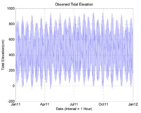
Time-series plot of the hourly tidal elevation at Incheon station.
Another way to determine the tidal parameters is to analyze a year of hourly observations of the levels. Many parameters may then be determined directly from the resulting harmonic constituents. Fig. 2 shows the line spectrum of harmonic constituents at Incheon.
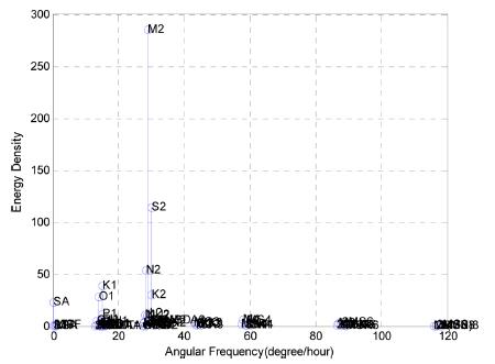
The line spectrum of the harmonic constituents at Incheon station.
Plants and animals have certain essential requirements (ecological niche), if they are to survive and prosper. Each organism has developed special characteristics to enable it to compete successfully in its particular environment; in particular, conditions on land and in water, and the species which live there, are very different. On the coast, certain species and ecosystems have developed to thrive in an environment that changes between these two extremes, in a pattern defined by the rise and fall of the tide (Swinbanks, 1982; Pugh, 2004; Hartnoll and Hawkins, 1982). For survival in this highly variable region, species must not only be able to cope with the relatively uniform conditions of submersion, but also with the varying periods of exposure to air. These periods of emersion, which may last for several hours, or at higher levels, days, must be survived until the next submergence.
Marine biologists have looked for relationships between the local tidal regime and the zonation of coastal species. The frequency distribution of tidal levels at coastal zones is in a form that allows them to be more easily related to particular levels of vertical zonation.
Recently, reliability or performance based design methods are adopted in the design of coastal structures, in which the distributional characteristics of design variables (e.g. mean and standard deviation of a variable of normal distribution) are important (Goda and Takagi, 2000). Therefore, it is necessary to provide the distributional characteristics of random design variables, for the reliable and optimal design of coastal structures. There are a number of variables related to coastal structure design using tidal data. In the present study, we deal with the harmonic and non-harmonic constants of hourly tidal level. Frequency distribution and emersion/submersion patterns at the tidal gauging stations in Korean coasts are also investigated. Finally, formulae for the estimation of the exposure duration in the inter-tidal zone are developed.
2. Materials and Methods
2.1 Materials
A number of tidal gauging (TG) stations and ocean monitoring stations now operated, starting from the Mokpo station in 1952 by the KHOA (Korea Hydrographic and Oceanographic Administration; http://www.khoa.go.kr/). The stations in operation can be classified, based on the coastal seas as six stations on the East coast, 17 stations on the South coast, and 23 stations on the West coast. Tidal elevation is continuously monitored, and these data are disseminated by using the annual tide table, ARS, Internet, and so on.
In this study, representative TG stations are selected to cover the whole Korean coastal seas, and the statistical parameters of the data in each TG station are analyzed. The TG stations are a total of eight stations: Incheon, Gunsan, Mokpo, Jeju, Yeosu, Busan, Pohang, and Sokcho stations, as shown in Fig. 3, and the basic information of the data is summarized in Table 1.
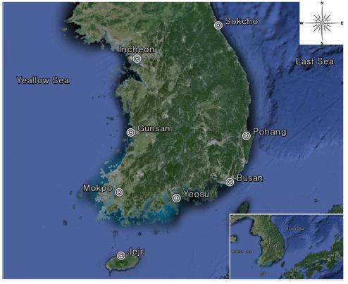
Location map of the tidal gauging stations on Korean coasts.

Location coordinates and data periods of the TG stations
2.2 Methods
The hourly tidal elevation (TE) data can be downloaded for only one-month period from the KHOA homepage (http://www.khoa.go.kr/). Each month, data sets are integrated as the continuous one year spreadsheet data. The data are plotted to check for missing periods and outliers, using the MATLAB program. After that, harmonic analysis of the data is performed, and frequency distributions and emersion-submersion curves are calculated. The parameters of the probability distribution function, having a form of the Gaussian mixture function, are optimally estimated using the least square method (Cho et al., 2004). The steps in the suggested modeling protocol are summarized in Fig. 4.
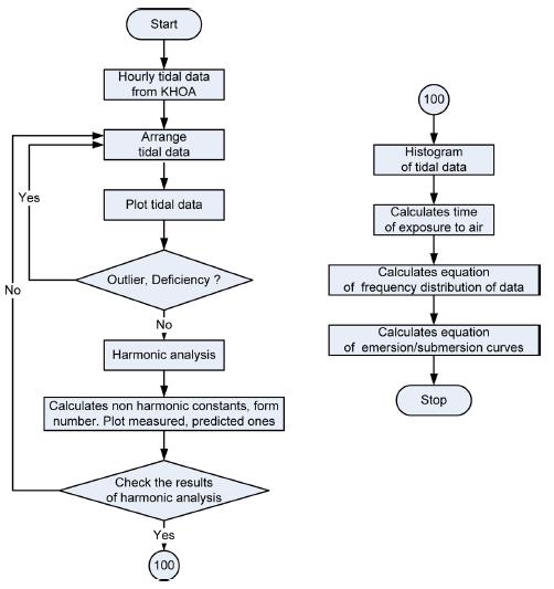
Steps of hourly tidal data analysis.
3. Harmonic Analysis of the Tidal Elevation Data
Harmonic analysis is the most commonly used method for tidal analysis, which treats the observed tides as the sum of a finite number of harmonic constituents, with periods of angular speeds determined from astronomical arguments. The vertical tide at any place can be expressed in terms of a sum of harmonic terms:
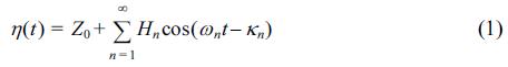
This expresses the heights, η(t), of the tide at any time, t. In Eq. 1, Z0 is the height of the mean water level above the datum used, and each cosine term is a tidal constituent. The amplitudes, Hn, of the constituents are derived from observed tidal data at a certain place. The frequency, ωn, is given in degrees per mean solar hour. The initial phase, κn, of the constituent is also determined from the observed tidal data. The number of constituents, n, is 65.
The relative importance of the diurnal and semidiurnal tidal constituents is sometimes expressed in terms of a tidal form number, F, derived from the harmonic constituent amplitudes:
We perform classical harmonic analysis using T_TIDE (Pawlowicz et al., 2002), which is written in MATLAB. Harmonic analysis results for the eight tidal gauging stations are summarized in Table 2.

Harmonic analysis results for the tidal gauging stations
When the form number is less than 0.25, we have semidiurnal tides - as in Incheon, Gunsan, Yeosu, and Busan TG stations. Between 0.25 and 1.5, tides are mixed, predominately semi-diurnal as in Mokpo, Jeju, Sokcho and between 1.5 and 3.0, mixed predominately diurnal - as in Pohang. Above 3.0, the tidal form is fully diurnal. We can see all different types of tide along the Korean coast.
The average spring high water level taken over a long period is called the High Water of Ordinary Spring Tide (HWOST), and the corresponding neap high water level is called the High Water of Ordinary Neap Tide (HWONT). The average spring low water level taken over a long period is called the Low Water of Ordinary Spring Tide (LWOST), and the corresponding neap low water level is called the Low Water of Ordinary Neap Tide (LWONT). The nontidal constants are summarized in Table 3.

Non-tidal constants of the tidal gauging stations (SR, NR, MR are the ranges in the spring tide, neap tide and mean-tide, respectively.)
4. Frequency Distributions and Emersion Curves
A histogram is a typical way to graphically summarize or describe a data set, by visually conveying its distribution using vertical bars. A histogram is obtained by first creating a set of bins or intervals that cover the range of the data set. There exist some common methods for choosing the bin width, h, most of which are obtained by trying to minimize the squared error between the true density and the estimate. We use the Normal Reference Rule, as follows (Martinez and Martinez, 2005).

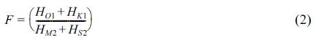
In Eq. (3), σ is the standard deviation of the TE data, and n is the number of the data (= 8,760 in this study). The total bin number is computed with ease, dividing the data range by bin width h. The frequency distributions of hourly tidal levels at the eight stations, which are shown in Fig. 5, are investigated using a histogram. We use the basic MATLAB package ‘hist’, which has a function for calculating and plotting a frequency histogram.
Histograms of the TE data.
The shape of the distribution in the Incheon and Gunsan TG stations, which are tide-dominated areas, shows a clear double-peak at HWONT and LWONT (bi-modal) in the distributions, and in the Mokpo station, shows an asymmetric double peak distribution. Whereas, the frequency distribution shape in the Jeju, Yeosu and Busan stations shows a smoothed flat peak, and in the Pohang and Sokcho stations, shows a single peak. Where the tidal regime is mixed, the use of Mean Higher High Water (MHHW) and Mean Lower Low Water (MLLW) becomes more appropriate.
In the meanwhile, the overall percentage of time for which each level is exposed to the air may also be presented statistically, using histograms. These percentage exposure plots are called exposure or emersion curves; it is easy to present the same statistics in the form of submersion or immersion curves. The extreme difference experienced by a species between emersion and submersion by the sea are presented statistically, as in Fig. 6.
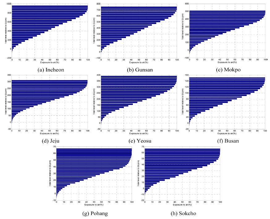
The exposure duration levels at Korean gauging stations.
5. Development of Exposure Duration Equation
5.1 Exposure Duration Equation
As shown in Fig. 5, for the semidiurnal tides there is a distinct double peak in the distribution. Cho et al.(2004) suggest Gaussian Mixture Distribution (GMD) as the probability density function of the tidal elevation data in the Korean coastal zone. In this case, the density function is given as follows;
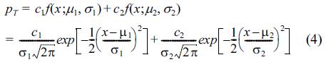
Eq. (4) expresses the double-peak distribution shape as the summation form of the two Gaussian distribution types, in which the different parameters, i.e. six parameters, are considered as scale parameters, of mean and variance. In these, c1, c2 are the scale parameters, which are dependent on the class interval, and accurately computed using the limitation that the integral sum for all intervals must be unity; the μ1, μ2 parameters could be considered as the means of each Gaussian distribution, and the σ1, σ2 parameters could be considered as the standard deviations of each distribution. The values of the μ1, μ2 parameters are nearly the same as the tidal elevation mode values, HWONT and LWONT. The detailed derivations of the scale parameters c1, c2 are given in the Appendix.
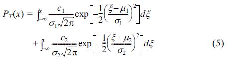
In this paper, an emersion/submersion curve equation is suggested as the integral of the frequency distribution of tidal levels. The emersion/submersion curve can be expressed using Eq. (5), as follows:
5.2 Parameter Estimation
Parameter estimation is a non-linear optimization problem constructed by RMSE (root-mean squared error) minimization. The problem is solved by the Levenberg-Marquardt method, modified by the Newton method (Bazaraa et al., 1993; Sec. 8.7). For the quantitative analysis, we compute the RMSE and R2 (coefficient of determination). The estimated results of the 6 parameters contained in the emersion/submersion curve, RMSE and R2 are shown in Table 4. Fig. 7 shows a comparison of the observed and proposed emersion/submersion curves, and we can see the emersion/submersion equations suggested in this study are accurate, and well fitted to the tidal elevation data. Note that R2 ≅ 1.0 provides a good fit.

Values of the optimal parameters, RMSE and R2
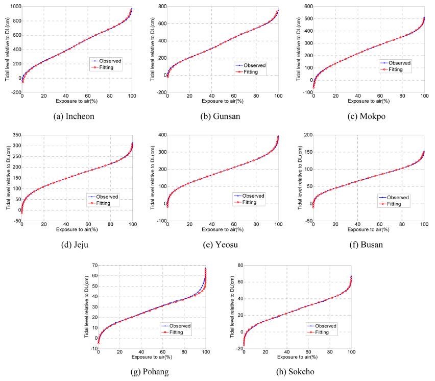
Comparison of the observed and fitted exposure duration curves.
Finally, the correlation analysis between non-tidal constants (Table 3) and the parameters of the exposure duration equation (Table 4) at each station are carried out. The scatter plot between parameters and non-tidal constants is displayed in Figs. 8-9.
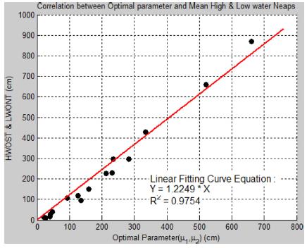
Relationship between μ1, μ2 parameters, and HWONT, and LWONT.
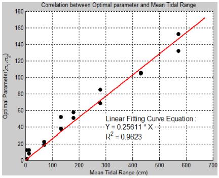
Relationship between σ1, σ2 parameters, and mean range.
The μ1, μ2 parameters are highly correlated to the LWONT and HWONT, and the σ1, σ2 parameters are also closely correlated to the mean tidal range, as shown in Fig. 8-9. The μ1, μ2 parameters coincide with the modes of the suggested probability distribution of the TE data. These can be regarded as the most frequently occurring TE values, because the LWONT and HWONT are the modes from the statistical point of meaning. Whereas, the σ1, σ2 parameters can be regarded as or related to the dispersion (or standard deviation) of the TE data, and also analyse the mean tidal range in terms of its physical meaning. In addition, it is clearly shown that the tidal phenomena are co-equal level, in the case of a symmetric distribution shape, and are ebbor flood-dominated, in the case of an asymmetric distribution shape, such as Mokpo TG station.
7. Conclusion
In this study, we investigate the harmonic and non-tidal constants, frequency distribution and emersion/submersion curves, using the hourly tidal data around the Korean Peninsula provided by the Korea Hydrographic and Oceanographic Administration (KHOA). The major findings of the study are as follows.
1) Harmonic analysis of the TE data is performed using the 65 tidal constituents. Harmonic and non-tidal constants analysis results for the eight representative tidal gauging stations are summarized. . Four tidal types (in practice, every tidal type) i.e. semidiurnal, mixed-mainly semidiurnal, mixed-mainly diurnal, and diurnal form, are observed along the Korean coast.
2) The shape of the frequency distributions of hourly tidal levels shows a distinct double peak for the semi-diurnal tides, and shows a single peak for the diurnal tides.
3) The extreme difference experienced by a species between emersion and submersion by the sea are presented statistically as the Cumulative Distribution Function(CDF) of the tidal elevation data.
4) An exposure duration equation is developed using Gaussian Mixture Distribution (GMD), and this shows good agreement with the observed data.
5) Correlation analysis between non-tidal constants, such as HWONT, LWONT and mean tidal range, and the parameters of the Gaussian mixture distribution is carried out, and the R2 values are 0.96-0.98.
Acknowledgements
This work was supported by the Manpower Development Program for Marine Energy, by the Korea Ministry of Oceans and Fisheries (MOF), and a study of the demonstration project for a 2.5 GW offshore wind farm at the southern part of the Yellow Sea, by the Ministry of Trade Industry and Energy (MOTIE).
References
Appendices
Appendix A: Derivation of the Scale Parameters, c1, c2 in the GMD Function
The scale parameters, c1, c2 of the Gaussian mixture distribution in Eq. (4) can be derived as follows :
On an assumption that the random variable, x follows some unknown distribution p(x) and the unknown distribution is regarded as a GMD function, the following conditions are satisfied.
If the sample mean is considered the population mean, it is as follows :

p(x) is defined as Eq. (A.2)

And, Eq. (A.3) is satisfied.

So, Eq. (A.4) can be derived by applying Eq. (A.2) and (A.3) to Eq. (A.1).
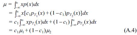
Eq. (A.4) is rewritten as Eq. (A.5)

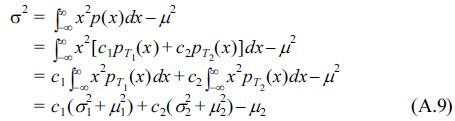
Similarly, scale parameters, c1, c2 can be defined by applying the above process to variance, that is, as follows :
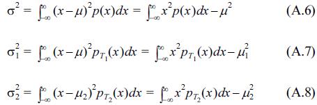
Substituting Eq. (A.2)~(A.3) and Eq. (A.7)~(A.8) into Eq. (A.6), the variance can be rewritten as Eq. (A.9).
Eq. (A.9) can be rearranged as Eq. (A.10)

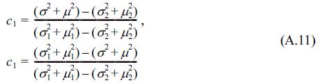
From Eq. (A.10), Eq. (A.11) is induced.