Characteristics of Tidal Current and Tidal Residual Current in the Chunsu Bay, Yellow Sea, Korea based on Numerical Modeling Experiments
수치모델링 실험을 통한 서해 천수만의 조류와 조석잔차류 특성
Article information
Abstract
This study is based on a series of numerical modeling experiments to understand the circulation and its change in the Chunsu Bay (CSB), Yellow Sea of Korea. A skill analysis was performed for the tidal height and tidal current of the observation data using the amplitude and phase of the 4 major tidal constituents respectively for verification of modeling experimental results. As a result, most of the skill score was seen to be over 90%, so numerical model experiment results can be said to be in good agreement with the observed tidal height and tidal current. Tidal wave proceeded from the entrance of the CSB towards inside, and the tidal range gradually increased to the north. It took about 10 to 30 minutes for the tidal wave to reach to northern end. The tidal wave showed a characteristic to rotate counter-clockwise in the southern part. The tidal current flowed to the north-south direction along the bottom topography; the angle of the major axis appeared alongside the isobath. It showed the characteristics of reversing tidal current with the minor axis less than 10% of the major axis. The strength of the tidal residual current that is influenced by geographical factors including bathymetry and coastline showed the range of 1~30 cm/sec, greater in the south channel and smaller in northern Bay. Two pairs of cyclonic/anti-cyclonic eddies around Jukdo and 3~4 pairs of strong eddies at the southern part of CSB in hundreds of m to a few km size by relative vorticity derived from the tidal residual current.
Trans Abstract
수치 모델링 실험을 활용하여 서해 천수만의 해수 유동과 그 변화를 이해하기 위한 연구를 수행했다. 모델링 실험 결과에 대한 검증을 위해 관측 자료의 조위와 조류 각각 4대 분조의 진폭과 위상을 이용하여 스킬 분석을 실시했다. 그 결과 스킬 점수는 대부분 90%가 넘는 것으로 보아 수치 모델링 실험 결과는 관측된 조위와 조류가 양호하게 일치하는 것으로 나타났다. 천수만의 조석파는 만 입구에서 안쪽으로 진행되며 북부로 갈수록 조차는 점차 증가했다. 조석파가 북부까지 도달하는데 약 10~30분의 시간이 소요되었다. 남부에서 조석파는 반시계 방향으로 회전하는 특성을 보였다. 조류는 해저 지형을 따라 남-북 방향으로 흘렀으며, 장축의 각도는 등수심선과 나란히 나타났다. 조류타원의 단축이 장축의 10% 이하로 왕복성 조류의 특성을 보였다. 수심과 해안선 등 지형적 요인에 의해 좌우되는 조석잔차류의 크기는 1~30cm/sec의 범위를 보였고, 남쪽 수로에서 컸으며 만의 북부에서는 작았다. 조석잔차류로부터 유도된 상대와도를 통해 수 백 m에서 수 km 크기로 시계/반시계 방향으로 회전하는 와류를 확인했고, 죽도 주변에서 2쌍, 남부에서 형성된 3~4쌍의 강한 와류 특성을 파악했다.
1. Introduction
The Chunsu Bay (hereafter, CSB) is a shallow back Bay with its water depth within 25 m located at 36o23'~36o37'N,126o20'~126o30'E, on the western central coast of Korea, surrounded by Anmyeondo of Taean-gun, Kanwoldo of Seosan, and the West Sea Line of Boryeong (Fig. 1). As the reclamation projects proceeded in Seosan A·B zone, the tidal embankment construction clapboard was completed in 1983~1985 and two major channels through the northern part of CSB were blocked; as a result the CSB area was reduced from 380 km2 to 180 km2 and the flow velocity near the tidal embankment has plunged down (So et al., 1998; Lee et al., 2011). This change of velocity field affected various marine environment variables; the production of fish, crustacean and mollusks was reduced by about 1/4 from the end of 1970s to the late 1990s, from the change of the marine environment and sediment due to the geographic variation according to the construction of the tidal embankment and the influx of eutrophic freshwater. In addition, it was reported recently that the summer stratification in CSB generated low-rise anoxic layer (hypoxia) and threatened the ecosystem (Lee et al., 2012).
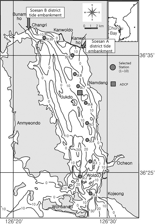
Map for the study area with locations for the various stations in the Chunsu Bay (CSB), Yellow Sea of Korea.
There are few researches until currently, however, on the physical process and characteristics in CSB and their impact to the ecosystem. Therefore, the importance of this study are as follows: first, the physical understanding of circulation (tidal current, density-driven current, and wind-driven current) with complex coastline and bottom topography considering the freshwater inflow from Kanwolho (hereafter, KW) and Bunamho (hereafter, BN), and the impact of the wind; second, understanding of changes in the ecosystem including eutrophication and the hypoxia, imminent regional issues from these geophysical processes.
The author has performing and reported a variety of researches recently for two years as follows by utilizing a numerical model in order to understand the physical characteristics of CSB with many of these issues. Hydrodynamic and hydrographic conditions in the CSB was observed and analyzed in detail using current meter records and water quality instrument by the present author (Jung et al., 2012b). Numerical modeling studies for the tide and tidal current in the CSB was also made by Jung et al. (2011a) and impact of the fresh water release on the circulation system in the CSB was investigated by Jung et al. (2011b, 2011c). Jung et al. (2012a, 2012b) also analyzed the salinity variation and stratification processes caused by freshwater release from the KW/BN based on numerical modeling study. Add to these results, Jung et al. (2012c) studied tracking patterns of freshwater using particle trajectory modeling experiments.
In the rapidly changing coastal marine environment, the inflow and behavior of freshwater, contaminants and other conservative substances are influenced by residual currents including the tidal residual current, wind-driven current and density-driven current (Yanagi, 1983). Therefore, in-depth researches are needed on the residual current influencing the net drift of substances in CSB that faces many problems in the marine environment and ecosystems in the summer due to the influx of a large amount of eutrophic freshwater from KW/BN. In the past, a variety of studies were performed in the world associated with the circulation in the coast and estuary on the characteristics of the tide and tidal current, and residual currents including wind-driven current and density-driven current, through observations and numerical models (Imasato, 1983; Goodrich et al., 1987; Dube et al., 1995; Guo and Valle-Levinson, 2008; Zhai et al., 2008); a variety of researches are also being conducted on the mechanism for the occurrence of residual currents (Kashiwai, 1984; Guo and Yanagi, 1996; Cai et al., 2003; Foreman et al., 2006).
In Korea, the physical researches on CSB were not much in the past 10 years compared to other Bays of Korea, except for a handful of papers including the study on the numerical modeling of circulation and diffusion of CSB and inshore of Yoo (1992), tidal phenomena change due to the tidal embankment construction of So et al. (1998), and CSB water quality prediction model development of Choi (2004). In this study, model configurations such as horizontal grid size, bottom topography, tidal constituents for model forcing and locations of open boundary, etc have improved compared to previous researches (Choi, 2004; Park and Oh, 1998; Seo et al., 1998; Yoo, 1992).
In this study, series of numerical modeling experiments were carried out and the results were analyzed to understand the tidal dynamics, the density-driven current caused by the freshwater discharge from the KW/BN tidal embankment, and the wind-driven current caused by the local wind. We intend to describe the results of intensive numerical modeling experiments in three separate papers in that in Paper 1, characteristics of tide and tidal current are analyzed in terms of tidal constituents; in Paper 2, the impact of summertime freshwater discharge on the modification of tidal current and its ellipse characteristics and change of 3D structure of salinity field; in Paper 3, the wind-driven current and its influence on the destratification of water column will be described. The objective of this paper is to analyze the characteristics of the tide, tidal current, and its residual current with associated vorticity field.
2. Numerical Model for the Chunsu Bay
2.1 Physical Setting and Bottom Topography
The CSB is located in the western coast of the Korean peninsula facing the Yellow Sea. It is a semi-closed north-south elongated bay blocked by the Seosan AB tidal embankment in the north. It is 25 km long by 8.5 km wide. The CSB is shallow with average depth of 10 m and maximum water depth is approximately 30 m at the entrance of the Bay shown in Fig. 1. A large amount of freshwater in two inland lakes (i.e., KW and BN) is discharged into the CSB during the summer season. Discharge rates for 3~4 hours were 400, 200 m3 /sec respectively. The annual 780 ×106m3 and 620 ×106m3 of freshwater entered the CSB from two tidal embankments (KW/BN) in 2010 and 2011 respectively. CSB is a typical shallow back bay with the bathymetry distribution ratio of 89.2% less than 20 m in water depth and 49.3% less than 10 m. As shown in Fig. 2 CSB was separated into northern, central, and southern regions.
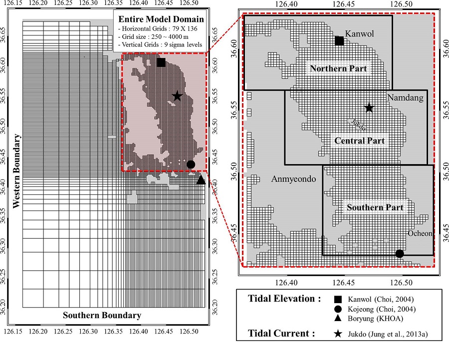
Grid system for the numerical model for the CSB, Yellow Sea of Korea. And location of datasets for model calibration and validation.
Jung et al. (2013a), observed the multilayer current speeds and directions at the center CSB in summer 2010 by the ADCP. The current speed was observed up to 40 cm/sec at surface, and the direction of the main flow was the NNESSW direction. The residual current flowed northward over the entire layers, with longer flow distance in the mid-layer than the surface, which seems to be due to the influence of fresh water (density-driven current) flowing south from the north of CSB. It is interpreted that the freshwater reached to the center of CSB and affected the circulation in 2~3 days from KW/BN lakes. CSB is the region with summer season monsoon climate, having prevailing southerly winds during the summer, and northwesterly winds prevailed in the winter. In addition, a large amount of fresh water flows in from KW/BN lakes in the summer monsoon season. The dynamics of the water circulation in CSB of is typically dominated by tides and tidal currents, but its impact varies depending on the effect of wind-driven current and density-driven current due to freshwater inflow. Influence of fresh water from KW and BN tide embankment in to the CSB and local wind-driven current will be of major subjects in the next papers.
2.2 Model Specification and Numerical Schemes
The numerical model for CSB estuarine used in this study is ECOM3D, a three-dimensional, sigma coordinate, hydrostatic, primitive equation model derived from Princeton Ocean Model (Blumberg and Mellor, 1987). No salt and heat flux conditions are applied to the surface boundary. At the bottom, the quadratic bottom stress with a bottom drag coefficient is applied with no salt and heat fluxes and zero vertical velocity. The costal wall boundary is impenetrable, impermeable and no-slip. A wetting and drying schemes was applied to the model, which defines dry-cells as regions with a thin water column of fluid 0 cm.
Characteristics of the model for this study are as follows. Freshwater flows in from KW/BN lakes in CSB north as in Fig. 1; seawater circulates with the offshore through the south channel. Wide-area grid was formed by extending the south and west boundaries, in order to minimize the problems that can occur when CSB entrance and the open boundary is close enough. 79 ×136 variable grids were constructed with horizontal grid size 250~4000 m for modeling; and CSB are configured with finer equal grids of 250 m for detailed understanding of the internal circulation in the Bay (Fig. 2). We used the mean sea level (MSL) data for model depth. In order to get a better understanding of the seawater circulation in the surface layer and the bottom layer, it was divided into 9 vertical sigma layers; most surface layer grids affected by the freshwater inflow were constructed with the vertical grid size of 0.5 m or less.
The initial condition of the modeling experiments was specified for the summer case with water temperature, 24.5oC, salinity, 31.0 (psu) obtained from on-site observations. Southern and western open boundary conditions were imposed by 4 major tidal constituents (M2, S2, K1 and O1) to force the tidal oscillation. Also the radiation boundary condition (Orlanski, 1976) was imposed at ebbing phase of model simulations. As shown in Table 1, the amplitude and phase of the 4 major tidal constituents were specified by using the tidal chart of NAO99 (Mastumoto et al., 2000). The amplitude of the M2 tidal constituent was given 1.98~2.16 m along the southern boundary, and 1.98~2.14 m along thewestern boundary. Model performances were evaluated based on the skill analyses in terms of tidal harmonics and tidal current ellipse parameters (not shown in this paper).

Amplitude (m) and phases (deg.) of tidal constituents used for model forcings at open boundary points
2.3 Field Measurements and Datasets for Model Calibration and Validation
Long time series of ADCP measurements at 14 levels with 1 meter vertical interval, for the period of 32 days from July 29 to Aug 30, 2010, (Jung, et al., 2012b, 2013a). Time series of measured surface current and its residual current at Jukdo station are shown in Fig. 3. In addition, a total of eight times field water quality surveys were conducted by using YSI6600, in terms of six parameters such as temperature, salinity, dissolved oxygen, chlorophyll, turbidity, and pH in 2010 and 2011, strong salinity stratification occurred in interlayer in summer; hypoxia water masses less than 3 ppm emerged in bottom layer; and dissolved oxygen oversaturation (120~160%) and chlorophyll a surge (up to 57 μg/L) phenomenon were observed in surface layer. The current and physical properties data were used as initial and boundary conditions, and validation data for the numerical modeling experiment of the study area (Fig. 1).
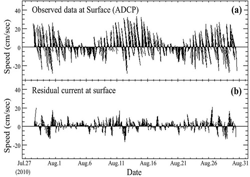
Time series of raw current meter records (a) and the residual current (c) at surface during Jul. 28~Aug. 30, 2010 at Jukdo Station.
Harmonic analyses were carried out to estimate tidal constituents and ellipse parameters by using the program package (Pawlowicz et al., 2002). Twenty tidal constituents were obtained by using 18-day record of one hourly sampled elevation and/or current components. The shortest and longest constituents resolved were M10 (2.48 hr) and MSF (354.37 hr) in our harmonic analyses.
3. Simulation of Tide and Tidal Current
3.1 Model Assessment and Validation
Three cases of numerical experiments were designed to understand 1) the basic tidal and tidal current characteristics in CS10TN case, 2) the impacts of the KW/BN freshwater release on the circulation system in CS10TD case and 3) added on the wind force and its effect in CS10TDW. In this paper, Part 1, only the results of Run CS10T are presented.
The verification of the model is indispensable before the modeling experiment. Among modeling experiment results, the verification of amplitude and phase of the tidal height and tidal current was performed using past observed tidal record (Jung et al., 2013a) and paper (Choi, 2004). The conditions of the open boundary were given using NAO99 data, but tidal height conditions of the open boundary was partly adjusted until the skill score (hereafter, SS) of M2, S2 tidal constituent becomes 85% or more at the stations of each validation.
To assess the model performance quantitatively, we adopt the skill score suggested by Martin and McCutcheon (1999) which is define as the deviation of the relative error from unity in the Eqn. (1).
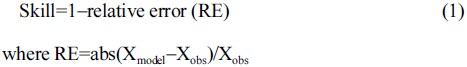
Here X can be any of characteristic parameters such as tidal amplitude, phase lag, or tidal ellipse parameters for the tidal elevation and velocity component.
Time series of sea level at the Boryung tidal station (Korea Hydrographic and Oceanographic Administration, abbreviated as KHOA) is shown in Fig. 4. To show the model performance of elevation to local tidal records (Boryung, KHOA), Kojeong and Kanwol (Choi, 2004)), SS of amplitudes and phase lags for the 4 major tidal constituents and are shown in Table 2. They show the average relative errors of 12.9% and 3.0% for the amplitude and phase lags, respectively. The skill scores demonstrate that the model performance is satisfactory. The tidal characteristics agree with previous works by Choi (2004).
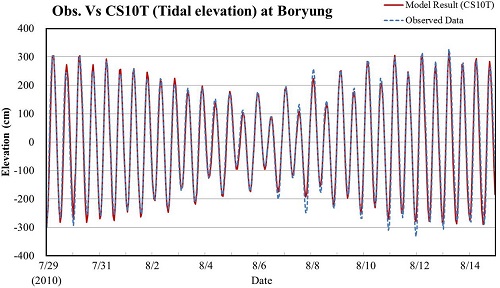
Time series of sea level elevation at Boryung Station in the CB. Elevation compared to model result (CS10T).

Comparison between model output and observations of sea level at three points in terms of 4 tidal constituents (unit: amplitude (m), phase (deg.) and skill score (%))
Time series of measured and model-computed surface current speeds at Jukdo station are shown in Fig. 5. Velocity components exhibit semi-diurnal oscillation with the spring-neap modulation in Fig. 5. The results of skill analyses of current in terms of the 4 major tidal constituents for the Jukdo station are shown in Table 3. The SS of amplitude and phase of M2 and S2 were greater than 90%. The amplitude and phase of K1 and O1 were around 70~78% and 60~90%, respectively. The diurnal constituents show higher correlation to density-driven current caused by the fresh water discharge, which will be simulated and analyzed in next paper.
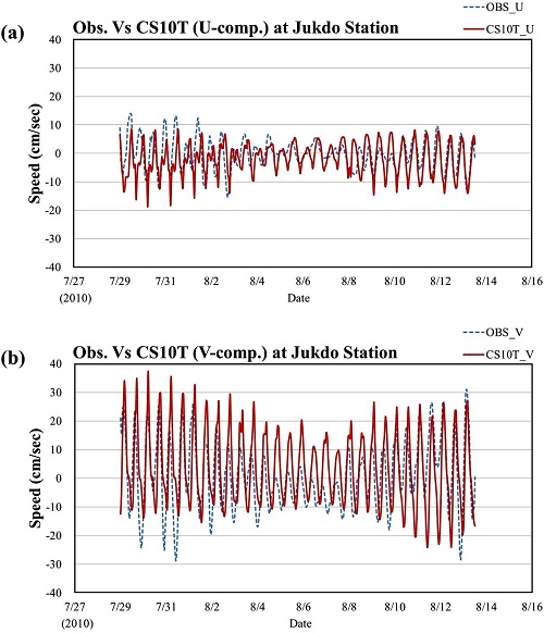
Time series of observed (ADCP) and model predict at Jukdo Station in the CB (a: U-component; b: V-component).

Comparison between model output and ADCP record for tidal current at Jukdo Station in terms of 4 tidal constituents (unit: amplitude (cm/s), phase (deg.) and skill score (%))
3.2 Simulation of Tide and Tidal Current
In Fig. 4, the time-series of the sea level shows the semidiurnal oscillation with fortnight modulation. The results of modeling experiments showed the spring range of 622 cm in Boryeong located at CSB entrance, 608 cm in adjacent Kojeong, and high 650 cm in KW north of CSB about 25 km away from Boryeong. The range at neap tide showed 210, 232 and 242 cm in Boryeong, Kojeong and KW respectively. Approximate Highest High Water (AHHW) was 728 cm in Boryeong, 718 cm in Kojeong and 760 cm in KW; High Water Ordinary Spring Tide (HWOST) was 675, 663 and 705 cm, respectively. In addition, High Water Ordinary Neap Tide (HWONT) was 469, 475 and 501 cm, respectively. KW, north of CSB showed larger spring and neap range than Kojeong, at the entrance of CSB by 42 and 10 cm, respectively. The tidal range gradually increases from the entrance to the northern limit of the CSB.
Fig. 6 show the tidal chart for the M2 and S2 constituents in the CSB. The amplitude of M2 and S2 tidal constituent showed arange of 202~223 cm and 93~112 cm, respectively. They show the increasing tendency towards the north from the bay entrance. On the other hand, the phase distributions show very complicated patterns near the entrance of the CSB probably due to the small islands. The phases of the M2 and S2 tidal constituent showed arange of 99~102o and 147~157o, in the southern part of Jukdo, respectively. The time lag from the entrance to the northern end is about 10~30 minutes. Simple calculation of the propagation velocity using 10 meter average depth will take around 33 minutes which agrees well with the phase difference in Figs. 6.
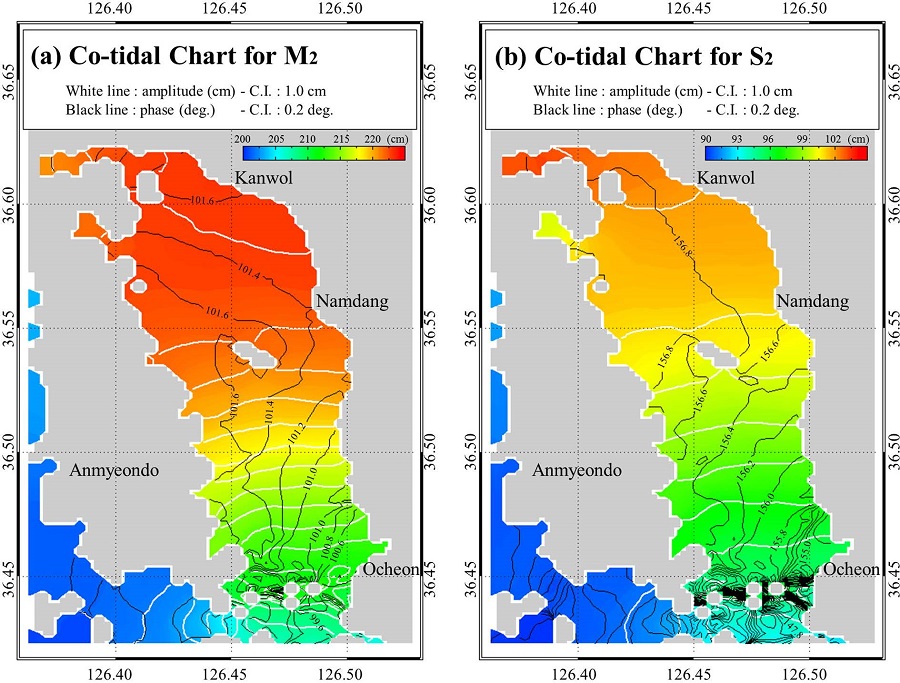
Co-tidal chart for M2 (a) and S2 (b) constituents in the CSB.
Tidal current in the CSB is complex due to a various geographical and physical factors such as the complex coastline, irregular bathymetry and open boundary. The northward velocity is approximately three times bigger than the east-west component at the central CSB, which is simply due to the fact that the CSB lying along the north-south. The current speed is fast at the south channel of the Bay entrance, but shows the gradual decrease towards the inner side of the Bay.
Fig. 7 show the horizontal distribution of simulated tidal current during flood/ebb of the spring/neap tide. The maximum ebb/flood current at spring tide shows the southward flow in Fig. 7a /northward in Fig. 7b. Both flood and ebb showed weak current velocity of 0.1~0.5 m/sec or less in the northern part, 0.3~1.5 m/sec at the central, 2~3 m/sec in the southern area; and a fast velocity of maximum 3~4 m/sec around the island at the Bay entrance. The horizontal distribution of maximum flood/ebb at neap tide is shown in Fig. 7c and 7d. The current speed showed approximately 3~8 times lower than the spring tide as 0.1 m/sec or less in the north part of the Bay, below 0.3 m/sec in the middle, and under 1.5 m/sec at the entrance of the Bay.
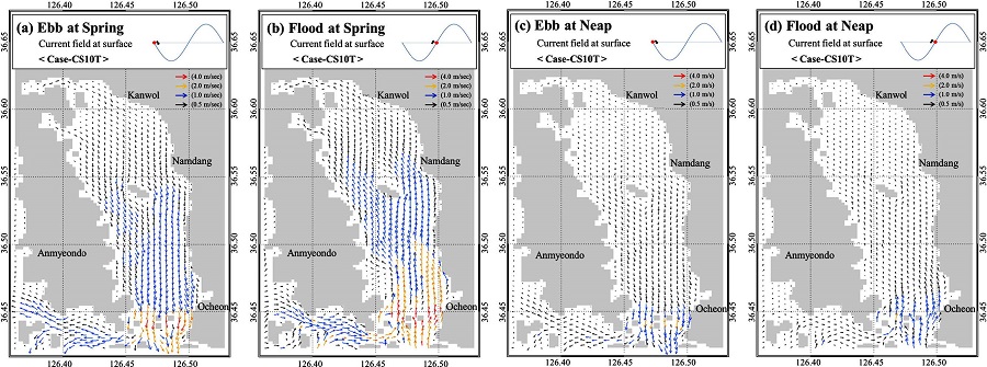
Horizontal distribution of the tidal current velocity field at spring ebb (a), spring flood phase (b) and neap ebb (c), neap flood phase (d).
Fig. 8 shows the horizontal distribution of the tidal ellipse for the M2 (a) and S2 (b) tidal constituents. Tidal ellipse characteristics of CSB can be summarized as follows. 1) Tidal current is recti-linear with ratio of minor/major axis very small less than 0.2. 2) The orientation of the major axis was in north-south direction along the isobath. 3) Around the Jukdo island, the current pattern shows more elliptical shape. 4) The major axis of the M2 tidal constituent was approximately 2 times bigger than that of S2. To represent the tidal ellipse parameters in the CSB, ten grid points are selected (Fig. 1) and Table 4 lists ellipse parameters in terms of semi-major, minor and inclination angle and phase lag for 4 major tidal constituents. Semi major axes for M2 tidal current range from 8.3 to 130.9 cm/sec, while semi minor axes for M2 from 0.6 to 9.6 cm/sec. Semi major axes for S2 tidal current range from 2.8 to 42.5 cm/sec, while semi minor axes for S2 from 0.5 to 9.4 cm/sec. At 10 stations, the angle of the major axis of the 4 tidal constituents shows the range of 74.4~129.4o in a counterclockwise direction around the x-axis.
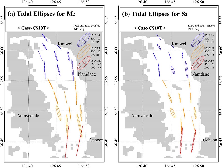
Horizontal distribution of tidal ellipses for M2 (a) and S2 (b) tidal constituents for the Case CS10T.

Tidal ellipse parameters for 4 major tidal constituents at selected ten grid points
3.3 Tidal Residual Current Field
Tidal residual current appears in the process of the tidal interaction with the terrain, and is known to generate and develop due to Coriolis Effect, friction, and advection terms (Robinson, 1983). Fig. 9 shows the horizontal distribution the 17-day average of tidal residual currents including both spring tide and ebb tide, of which the distribution patterns are very complicated. The pattern of tidal residual current can be summarized as follows. 1) The velocity range of the residual current in northern CSB is 1~7 cm/sec, and a large 10~30 cm / sec in the south. 2) Paired in clockwise/counterclockwise direction, several tidal residual currents exist near Jukdo at the central CSB at a velocity of 5~15 cm/sec, and at the southern entrance to CSB at 20~30 cm/sec. Paired eddy will be discussed next in vorticity characteristics. 3) Similarly to the previous study results of So et al. (1998) and Choi (2004), northwestern flows are present along the coast in the waters near KW/BN seawall north of CSB. 4) Overall, mostly northward flows were dominant in eastern CSB, and southward flows were dominant in the west. 5) Northward residual current is distributed mostly in the middle of the Bay, and southward tidal residual current is distributed along the coast. 6) The tidal residual currents appear largely around islands. This pattern is deeply related with tidal residual currents generated by flows, past specific structures such as islands or breakwaters, studied by Imasato (1983) and Robinson (1981).
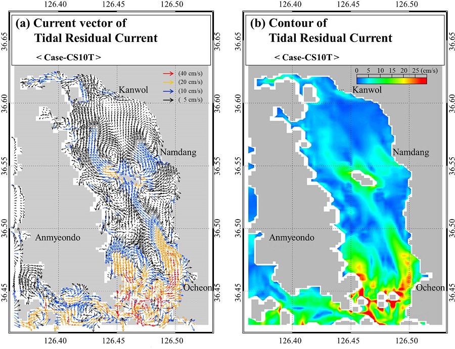
Horizontal distribution of tidal residual current field in the CSB at surface.
Table 5 is a summary of the basic statistics of 10 stations among tidal residual currents of the model run CS10T. In average residual currents, u-component range showed −6.0 ~12.6 cm/sec, and v-component range, 0.7~18.3 cm/sec respectively. Except for the residual currents with smaller size, the standard deviation of the u- and v-components were noticeable 1.1~3.8 and 1.8~13.3 respectively, which indicate that the tidal residual currents have greater the variations. Especially in stations 1 and 2 at CSB south, the v-comp has reached the maximum of 51.1 and 47.7 cm/sec respectively. Through the results of the average tidal residual current, the flood/ebb imbalance can be assumed to be dominated by geographic factors.

Basic statistics of tidal residual current of model run CS10T at the selected points
Vertical component of relative vorticity (hereafter, RV) is expressed in Eqn. (2)
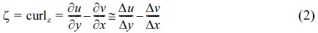
In computation of RV, we estimated it by using center-finite difference scheme.
The horizontal distribution of the tidal residual current shown in Fig. 9 and the RV of Fig. 10 are highly relevant. In Fig. 10a, the red means cyclonic and the blue means anti-cyclonic eddy. RV range is −40×10−5~40×10−5 sec−1; (-) indicates anti-cyclonic and (+), cyclonic direction. Fig. 10b shows some patterns of eddy paired cyclonic and anti-cyclonic. Around Jukdo at central CSB, a total of 4 major eddies, 2 cyclonic and 2 anti-cyclonic, are present; and 2 small eddies are surrounding them. 3~4 pairs of main eddy exist as very strong flows in CSB south. From the flow direction of the tidal current in the CSB, cyclonic (+) eddy was formed when bathymetry deepens, anti-cyclonic (-) eddy was formed when shallow; anti-cyclonic eddy was formed in the southeast and northwest of the island, and cyclonic eddy was formed in southwest and northeast. This eddy formation in the CSB is consistent with the eddy formation from bathymetry changes and seabed friction proposed by Robinson (1981) and Maze et al. (1998), and with the eddy formation around the headland suggested in the study of Zimmerman (1979, 1981), Signell and Harris (2000).
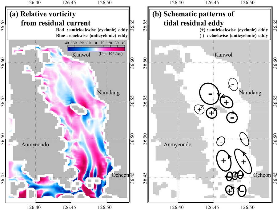
Horizontal distribution of relative vorticity from residual current (a) and schematic patterns of tidal residual eddy (b) in the CB at surface.
4. Discussion and Summary
In this study, numerical modeling experiments were carried out in order to understand the characteristics of tide and tidal current, and its residual current. The model results were validated with the measured data for the validation of modeling experimental results, which were verified through skills analysis using the amplitude and phase of 4 major tidal constituent (M2, S2, K1 and O1) of current velocity and sealevel. The results of skill analyses for the 4 major tidal constituents of sea level showed that mostly 90%, and the phase, 95%. The results of skill analyses for tidal current for M2, S2 tidal constituents shows higher than 90%, while those for K1 and O1 constituents were around 70~78% and 60~90%.
The characteristics of the tidal height of CSB were able to be understood through tidal height time-series of Fig. 4, and co-tidal chart in Fig. 6. Tidal height fluctuations of CSB showed the characteristics of spring-neap with two week-periods, and characteristics of semi diurnal tide. The tidal wave propagates from the entrance of the Bay towards the inside, and rotates counter-clockwise in the southern part of CSB. Tidal range was gradually increased towards KW/BN. For each tidal constituent, time lag of tidal wave showed between 10 to 30 minutes from the Bay entrance to the northern end.
As for CSB tidal current, south-north direction of the flow was dominant along the seafloor topography, with fast flow of 2~3 m/sec at the narrow waterways of the CSB entrance. The farther north of CSB, the flow rate significantly reduced compared to southern part. According to the analysis result of the tidal ellipse of the 4 major tidal constituents, the minor axis was under the size of 10% of the major axis, showing the characteristics of reversing tide, with the angle of the major axis side-by-side with the isobath. In CSB, the size of the M2 tidal constituent was about twice larger than S2 tidal constituent.
In CSB, the size of the tidal residual current was 1~7 cm/sec in the northern part and 10~30 cm/sec in the South, with the distribution very complex, and largely dependent on the geographic factors including bathymetry and coastline. The tidal residual current tends to flow towards the northwest along the KW/BN tidal embankment in northern part, but much smaller than at the entrance. Several tidal residual currents were paired cyclonic/anti-cyclonic. Characteristics of the eddy rotation were examined through relative vorticity derived from the tidal residual current. Among several eddies, with the size of hundreds of m to a few km, that were formed by bathymetry changes, seabed friction, and certain structures, 2 pairs of cyclonic/anti-cyclonic major eddies were shown nearby Jukdo in the CSB center, and 3-4 pairs of strong major eddies were formed in the south. Small eddy that occurs locally has a very high correlation with the formation of tidal residual current.
CSB is the Bay with a variety of geographic variation for over 30 years such as shoreline changes, bathymetry and volume changes due to reclamation projects. These problems are closely related to the changes in tidal phenomena due to KW/BN tidal embankment construction that So et al. (1998) studied, and also have a close relationship with changes and reduction of biota due to eutrophic inflow of fresh water that Lee (1996) and Lee et al. (1997) suggested, and with the generation of bottom layer hypoxia stratification in summer that Lee et al. (2012) reported. Based on the numerical modeling experiments, we understand tide, tidal current and tidal residual current in the CSB; and is such as density-driven current formation from the influx of freshwater from KW/BN, salinity field changes and stratification, and wind-driven current due to the influence of local winds. Understanding these physical processes will lead to help solve more complicated issues such as changes in water quality, and formation of hypoxia, degradation of the ecosystems, etc. that the CSB currently suffer from.
Acknowledgements
This research was a part of the project titled ‘2011 ChungCheong Sea Grand Program’ funded by the Ministry of Oceans and Fisheries, Korea. The authors thank anonymous reviewers for their helpful comments.